| Description |
Support vector machines were developed by Vapnik et al. based on the Structural Risk Minimization principle from statistical learning theory. They can be applied to regression, classification, and
density estimation problems.
Vapnik's book "Statistical Learning Theory" is
listed under "Publications", above.
Focussing on classification, SVMs take as input an i.i.d. training
sample Sn
(x1,y1),
(x2,y2), ...,
(xn,yn)
of size n from a fixed but unknown distribution Pr(x,y)
describing the learning task. xi represents the
document content and yi ∈ {-1,+1} indicates the
class.
In their basic form, SVM classifiers learn binary, linear decision rules
h(x) = sign(w *x + b) =
- +1, if w * x + b > 0, and
- -1, else
described by a weight vector w and a threshold b. According to
which side of the hyperplane the attribute vector x lies on,
it is classified into class +1 or -1. The idea of structural risk
minimization is to find a hypothesis h for which one can guarantee
the lowest probability of error. For SVMs, Vapnik shows that this
goal can be translated into finding the hyperplane with maximum
margin for separable data, this is depicted in the following figure.
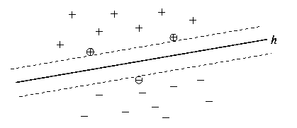
For separable training sets SVMs find the hyperplane h, which
separates the positive and negative training examples with maximum
margin. The examples closest to the hyperplane are called Support
Vectors (marked with circles).
Computing this hyperplane is equivalent to solving the following
quadratic optimization problem (see also algorithms).
minimize: W(α) =
|
n |
|
n |
n |
|
| - |
∑ |
αi + 1/2 * |
∑ |
∑ |
yiyjαiα
j(xi *
xj)
|
|
i=1 |
|
i=1 |
j=1 |
|
subject to:
| n |
|
n |
|
| ∑ |
yiαi = 0, |
∀ |
: 0 < αi
< C |
| i=1 |
|
i=1 |
|
Support vectors are those training examples xi with
αi > 0 at the solution. From the solution of this
optimization problem the decision rule can be computed as
|
n |
|
| w * x = |
∑ |
αiyi
(xi * x) and b = yusv -
w * xusv |
|
i=1 |
|
The training example (xusv,yusv) for
calculating b must be a support vector with αusv
< C.
For both solving the quadratic optimization problem as well as
applying the learned decision rule, it is sufficient to be able to
calculate inner products between document vectors.
Exploiting this property, Boser et al. introduced the use of kernels
K(x1,x2) for learning non-linear
decision rules.
Popular kernel functions are:
| Kpoly (d1,d2) |
= (d1 * d2 + 1)d |
| Krbf (d1,d2) |
= exp(γ (d1 - d2)2 ) |
| Ksigmoid (d1,d2) |
= tanh( s(d1 * d2) + c ) |
Depending on the type of kernel function, SVMs learn polynomial
classifiers, radial basis function (RBF) classifiers, or two layer
sigmoid neural nets. Such kernels calculate an inner-product in some
feature space and replace the inner-product in the formulas above.
A good tutorial on SVMs for classification is "A Tutorial on
Support Vector Machines for Pattern Recognition", for details,
please follow the corresponding link above. |