Glossary

Accuracy

The Accuracy is a standard measure to evaluate the quality of hypotheses in the context of concept learning.

Hypotheses are classifiers, determining if instances of an underlying universe of discourse belong to a specific concept or not. Algorithms addressing the task of concept learning usually output such a hypothesis after processing a given training set. A training set consists of classified instances, i.e. it is given if instances belong to the target concept or not.

To estimate the quality of such a hypothesis, another set, a so called test set, is separated from the set of available (classified) examples, and the learning algorithm is only provided with the remaining examples. Afterwards the (yet unseen) examples of the test set are classified by the hypothesis and the predicted class of each instance is compared to the correct one. The accuracy is the ratio of correct classified instances to number of instances in the test set.

more...

AdaBoost

AdaBoost is a boosting algorithm, running a given weak learner several times on slightly altered training data, and combining the hypotheses to one final hypothesis, in order to achieve higher accuracy than the weak learner's hypothesis would have.

The main idea of AdaBoost is to assign each example of the given training set a weight. At the beginning all weights are equal, but in every round the weak learner returns a hypothesis, and the weights of all examples classified wrong by that hypothesis are increased. That way the weak learner is forced to focus on the difficult examples of the training set. The final hypothesis is a combination of the hypotheses of all rounds, namely a weighted majority vote, where hypotheses with lower classification error have higher weight.

In detail:

Given

a set E = { (x₁, y₁), ..., (x_n, y_n) } of classified examples, where x_i ∈ X and y_i ∈ Y, for i = 1, ..., n. Here we assume Y = {-1, +1}, e.g. instances that are not covered by a concept to be learned have label -1 and the ones covered have label +1.
a weak learning algorithm that can deal with weighted example sets. Such a learning algorithm reads an example set E and a distribution D. In the most simple case, where all hypotheses that can be output are functions X → {-1, +1}, the algorithm tries to find a hypothesis h with minimal probability of misclassification, given that an example is drawn from X with respect to D. The case of other possible hypotheses can be addressed by using more complex error measures.

The algorithm:

Let D_t(i) denote the weight of example i in round t.

Initialization: Assign each example (x_i, y_i) ∈ E the weight D₁(i) := 1/n.
For t = 1 to T:
- Call the weak learning algorithm with example set E and weight s given by D_t.
- Get a weak hypothesis h_t : X → ℝ.
- Update the weights of all examples.
Output the final hypothesis, generated from the hypotheses of rounds 1 to T.

Updating the weights in round t:

D_t+1(i) := D_t(i) * exp(α_ty_ih_t(x_i)) / Z_t , where

Z_t is chosen such, that D_t+1 is a distribution.
α_t is chosen according to the importance of hypothesis h_t. For h_t: X → {-1, 1} usually α_t is chosen as
α_t := 1/2 * ln ( (1 - ε_t) / ε_t ),
where ε_t denotes the classification error of hypothesis h_t.

The final hypothesis H: X → {-1, +1} is chosen as

	_T
H(X) = sign(	∑	α_th_t(x) ).
	^t=1

For more details, please refer to the publication link above. more...

Agents

Intelligent agents are possibly mobile programs that optimize their behavior according to a given performance measure.
Also operators of a knowledge discovery process haven been implemented in the form of software agents.

more...

Algorithmic issues

more...

Analysis tasks for resource management, quality control and decision making

Analysis tasks for resource management, quality control and decision making are demanded by the health sector.

more...

APRIORI

APRIORI provides a solution for a subtask of Association Rule Learning.

The subtask can be stated as follows:

Find all sets of items (itemsets) that have transaction support above minimum support. The support for an itemset is the number of transactions that contain the itemset. Itemsets with minimum support are called large itemsets.

We use the following notation:

Let I = {i₁, i ₂,...,i_m} be a set of literals, called items.
Let D be a set of transactions, where each transaction T is a set of items such that T ⊆ I.
Let X be a set of items in I. A transaction T is said to contain X, if X ⊆ T.

Discovering large itemsets

Discovering large itemsets requires making multiple passes over the data.

In the first pass, we count the support of individual items and determine which of them are large, i.e. have minimum support.
Each subsequent pass starts with a seed set of itemsets found to be large in the previous pass. This seed set is used for generating new potentially large itemsets, called candidate itemsets.
The actual support for these candidate itemsetsis counted during a new pass over the data.
At the end of the pass, we determine which of the candidate itemsets are actually large. These itemsets become the seed for the next pass.
This process continues until no large itemsets are found.

If the fraction of transactions belonging to large itemsets becomes small, it will be more efficient to store their transaction IDs and just work on that subset, than to perform passes over the complete dataset.

Algorithm APRIORI

Notation:

k-itemset An itemset having k items.
L_k Set of large k-itemsets (those with minimum support).
C_k Set of candidate k-itemsets (potentially large itemsets).

L₁={large 1-itemsets};
for (k=2; L_k-1 ≠ ∅; k++) do begin
C_k=apriori-gen(L_k-1); // New candidates
forall transactions t ∈ D do begin
C_t = subset( C_k,t); //Candidates contained in t
forall candidates c ∈C_t do
c.count++;
end
L_k = {c ∈ C_k | c.count ≥ minsup}
end
Answer=U_k L_k

The apriori-gen function takes L_k-1, the set of all large (k-1)-itemsets, as an argument, and returns a set of candidates for being large k-itemsets. It exploits the fact, that expanding an itemset will reduce its support. A k-itemset can only be large, if all of its (k-1)-subsets are. So apriori-gen generates only candidates with this property, which can easily be achieved given the set L_k-1.

more...

AQn

The family of AQ-Algorithms provides methods for concept learning and conceptual clustering. This section just introduces some base functionality. For more information, please follow the links.

AQ applied to Concept Learning
AQ learns concepts from a set P of positive examples and from a set N of negative examples by the following loop: Choose a single p ∈ P, generalize it as much as possible, so that no n ∈ N is covered and remove all covered positive examples from P. This is done until the disjunction of the generalized examples covers every p ∈ P.

Algorithm:
- Set K := ∅.
- The set P consists of all positive examples.
- Repeat, until P is empty:
  - Choose an example p ∈ P.
  - Generate STAR({p}|N), a list of maximally general conjunctive descriptions, separating p from all elements of N.
  - Choose a best element b of STAR({p}|N). The quality is measured by a "Lexical Evaluation Function".
  - Set K := K ∪ {b}.
  - Delete all p from P, that are covered by b.
- Output the disjunction of all elements of K.
AQ applied to Conceptual Clustering
Following the star-method, one possibile way to build clusters is to (e.g. randomly) choose a subset of all given observations, and to distinguish each of its elements from all of the other elements of the subset.

Algorithm:
Given a set of observations E.
- Choose a subset K ⊆ E.
- For each e ∈ K generate STAR({e}|K\{e}) to distinguish e from all other elements of K.
- Choose and specialize the best concept definitions given by the stars, such that every possible observation is covered by at most one concept. This process is guided by a "Lexical Evaluation Function" (LEF), measuring the quality of concepts.
- If the generated concepts do not fit the given requirements, another run with a different subset of E may be necessary.
- If a partition is suitable according to the LEF, concepts may be refined. This is done by splitting the set of all observations, covered by a single concept, by another run of the clustering algorithm, in order to induce a hierarchy of concepts.

more...

Association Rule Learning

Association rules describe correlation of events and can be regarded as probabilistic rules. "Correlation of events" means, that events are frequently observed together. Discovering association rules in large databases can be a first step of knowledge discovery in databases (KDD).

A good example from real life are databases of sales transactions, which have become an important part of marketing infrastructure of many companies. Knowledge about sets of items frequently bought together helps these companies to develop successful marketing strategies.

more...

Attribute-Value

If a learning algorithm uses an attribute-value representation, each instance of the underlying universe of discourse is described by the values of a given set of attributes, as common in relational databases. Each attribute can be regarded as a function, mapping the universe of discourse to a specific domain.

If we say the example language of a learning algorithm is an attribute-value representation, without specifying the type of attributes, we usually mean, that the domain of each attribute is finite or nominal and each value is treated by the learning algorithm without using a specific interpretation. In contrast, if we talk about numerical attributes, we often think of attributes having infinite domains with a natural interpretation a learning algorithm may use.

more...

Audio categorisation

more...

AutoClass

AutoClass is an unsupervised Bayesian classification system that seeks a maximum posterior probability classification. Its inputs consist of a database of attribute vectors (cases), either real or discrete valued, and a class model. Default class models are provided. AutoClass finds the set of classes that is maximally probable with respect to the data and model. The output is a set of class descriptions, and partial membership of the cases in the classes.

Please follow the link above to download the sourcecode for Windows or Unix platforms. more...

Bayes Theorem

Bayes Theorem provides a method for calculating P(h | D), denoting the probability of h being correct, given a specific data set D.

Let

P be a probability distribution,
h be a hypothesis and
D be a data set.

If we know

P(h), the probability of hypothesis h being correct,
P(D), the probability of data set D being observed, and
P(D | h), the probability of observing D, under the assumption of h being correct,

then Bayes Theorem provides a method for calculating P(h | D), denoting the probability of h being correct, given a specific data set D.

Bayes Theorem:

P(h | D) = P(D | h) * P(h) / P(D)

An application of Bayes Theorem:

Given a data set D, find a hypothesis h ∈ H with highest posteriori probability P(h | D).
Method: Chose a hypothesis h ∈ H that maximizes the expression P(D | h) * P(h).

more...

Bayesian Learning

Bayesian Learning constitutes a probabilistic view of learning, based on Bayes Theorem. The underlying assumption is, that there is a set of hypotheses, each having a certain probability of being correct. Receiving more information changes the probabilities from a learner's point of view. For instance an observation might contradict a hypothesis, or strengthen the belief in it. The aim in this setting is to be able to find a hypothesis with highest probability of being correct, given a specific set of data / piece of information.

Bayes Theorem:

Let

... P be a probability distribution.
... h_i, i ∈ {1, ..., n} denote a set of hypotheses.
... P(h_i) denote the probability of h_i being correct in the general case, that is without being given any additional information. P(h_i) is called the prior probability of h_i.
... D denote a set of data.
... P(D) be the probability of the information denoted by D being correct in the general case.
... P(D | h_i) denote the probability of the information D being correct, given the correctness of hypothesis h_i.
... P(h_i | D) denote the probability of the correctness of hypothesis h_i, given the additional information D. This is called the posterior probability of hypothesis h_i.

Bayes Theorem:

P(h | D) = P(D | h) * P(h) / P(D)

This theorem allows us to find a hypothesis h'with maximum posterior probability, given the prior probabilities of all hypotheses and the probabilities of D being correct under the assumption of each single hypothesis being correct:

h' := max [ P(D | h_i) * P(h_i) ]

^h_i

more...

Bayesian Networks

A Bayesian network or Bayesian belief network is a directed acyclic graph of nodes representing variables and arcs representing dependence relations among the variables. If there is an arc from node A to another node B, then we say that A is a parent of B. If a node has a known value, it is said to be an evidence node. A node can represent any kind of variable, be it an observed measurement, a parameter, a latent variable, or a hypothesis. Nodes are not restricted to representing random variables; this is what is "Bayesian" about a Bayesian network.

A Bayesian network is a representation of the joint distribution over all the variables represented by nodes in the graph. Let the variables be X(1), ..., X(n). Let parents(A) be the parents of the node A. Then the joint distribution for X(1) through X(n) is represented as the product of the probability distributions p(X(i) | parents(X(i))) for i from 1 to n. If X has no parents, its probability distribution is said to be unconditional, otherwise it is conditional.

Questions about dependence among variables can be answered by studying the graph alone. It can be shown that the graphical notion called d-separation corresponds to the notion of conditional independence: if nodes X and Y are d-separated (given specified evidence nodes), then variables X and Y are independent given the evidence variables.

In order to carry out numerical calculations, it is necessary to further specify for each node X the probability distribution for X conditional on its parents. The distribution of X given its parents may have any form. However, it is common to work with discrete or Gaussian distributions, since that simplifies calculations.

The goal of inference is typically to find the conditional distribution of a subset of the variables, conditional on known values for some other subset (the evidence), and integrating over any other variables. Thus a Bayesian network can be considered a mechanism for automatically constructing extensions of Bayes' theorem to more complex problems.

Bayesian networks are used for modelling knowledge in gene regulatory networks, medicine, engineering, text analysis, image processing, and decision support systems.

more...

Best Region Rules

The Best Region Rules algorithm addresses the task of predicting the occurence of future events on the basis of past events.

The hypotheses of the algorithm are specific rules:

Each rule contains a condition, a target and a lag interval. The interpretation of such a rule is, that target events occur with a delay, lying within the given time interval, after condition events. The rule A[5, 20] => B would e.g. have the interpretation "B occurs between 5 and 20 time units after occurences of A".

Measuring the Quality of a Rule

For specific applications, the intuitive quality measure of rules can vary, so the algorithm offers different measures, which are weighted by the user. The easiest of these measures are Prediction Accuracy and Recall Accuracy.

For a specific event sequence the Prediction Accuracy of a rule is defined as the ratio of

condition events, followed by a target event within the given intervall
to all condition events.

The Recall Accuracy is defined very similar. It measures the ratio of

target events following a condition event with a delay in the given interval,
to all target events.

These definitions basically reflect the usual meaning of accuracy and recall. Further measures reward beneficial properties of rules, like smaller interval regions, higher predictive power, or multiple hits (e.g. multiple target events matching a single condition event).

Finding Good Rules

The search for good rules is limited to Minimal Regions. With respect to a given lag set Minimal Regions are minimal lag intervals, covering the lags of a specific subset of event pairs. Limiting the search to such regions is resonable, considering that there are no negative examples in a event sequence, and that usually larger regions will be assigned higher quality scores.

The algorithm will first calculate all occuring time lags between different event types of a given event sequence.
If event A occurs at time points 5, 10 and 20 and event B occurs at 11, 15 and 21, then the resulting lag set is {1, 5, 6, 10, 11, 16}.

The algorithm will choose all minimal regions for generating rule candidates.

In the example above the rules with condition event A, target event B, and Minimal Regions are:
A[1, 1] => B, A[1, 5] => B, A[1, 6] => B, ..., A[1, 16] => B
A[5, 5] => B, A[5, 6] => B, ..., A[5, 16] => B
...
A[16, 16] => B

For learning models from event sequences the Best Region Rules algorithm can calculate the best Minimal Region for each event pair, according to a given quality measure (weights of the algorithm's measures). All best rules, exceeding a minimal quality score, form the hypothesis.

more...

Boosting

The notion of Boosting subsumes methods of improving learning algorithms. If learning algorithms fail to provide arbitrarily good results for a specific concept learning task, i.e. they fail to output arbitrarily good hypothesis with arbitrary high probability, they often can be "boosted" to perform much better.

In the PAC-learning scenario the following is required for a learning algorithm A:

For arbitrary δ and ε greater than 0, and
for each target concept c of a given hypothesis language LH,

A has to be able to choose a hypothesis,

approximating c ε-good,
with a probability of at least (1 - δ),
after reading a random training sample of size polynomial in (1 / δ) and (1 / ε).

Please follow the link to "PAC-Learning", for more details.

The requirements of PAC-Learning are strong, and usually do not hold in practice for common learning algorithms. Instead one has so called weak learners, performing just slightly better than random guessing.

A weak learning algorithm manages

for each target concept of a given hypothesis language, to
output a hypothesis with error below 1/2 - p(|E|),
with a probability greater than 0,
provided with a random training sample,

where p is a polynomal.

The aim of boosting is to improve the accuracy (1 - ε above) reached by a weak learner, and to reduce the probability of outliers (δ above), i.e. that random samples lead to bad hypothesis.

Therefore boosting algorithms ...

run a given weak learner several times, where each round either the set of examples is slightly altered, e.g. by shifting the weight of examples, or the algorithm is allowed to read new examples each time.
combine the set of hypotheses to one final hypothesis, e.g. by using a weighted majority vote.

more...

Bootstrap

Bootstrapping provides a method to estimate the quality of a concept learning algorithm (classifier).

Draw from the data set a new data set with replacement, the sample being of the same size as the data set. Typically, 1/e = 37% of the original data set will be unused in the drawn data set.

Train the classifier on the drawn set, and estimate the error on the unused parts. Averaging the performance on a large number of experiments gives the final estimate.

more...

Bottom-Up Induction of Horn Clauses

A method to induce horn clauses in Inductive Logic Programming,

covering a given set of positive examples, but
being as specific as possible,

is to perform a bottom-up search through the hypothesis language.

Scenario:

All examples are ground facts with the same predicate symbol and arity.
Background knowledge B may be given in the form of other, extensionally defined predicates.
The first example may be considered as a first hypothesis.
Whenever a new example is read, that cannot be derived from the background knowledge and the actual horn clause, a generalization step has to be performed.

So the generalization step leads from an insufficiently general horn clause h to another horn clause h':

If an example can be derived from B and h, then this example can be derived from B and h´ as well.
Additionally the new example can be derived by h´.

To find such a hypothesis h´ the least general generalization and the inverse resolution provide suitable procedures. An algorithm using these procedures is GOLEM. more...

C4.5

C4.5 (Quinlan) is an extension of the base algorithm ID3.

Some of the additional features are:

incorporation of numerical (continous) attributes
nominal (discrete) values of a single attribute may be grouped together, to support more complex tests
post-pruning after induction of trees, e.g. based on test sets, in order to increase accuracy
C4.5 can deal with incomplete information (missing attribute values).

Please refer to the link above for software. more...

CANDIDATE-ELIMINATION

The versions space consists of all actual generalizations, all actual specializations and the hypotheses "in between". Intuitively spoken the versions space is the set of the remaining hypotheses still consistent with the given examples and is described by the set of most general and by the set of most specific hypothesis. As soon as both sets intersect, a target concept is within the intersection. Supplying more examples will lead to identical sets. All concepts in this set are possible solutions. To continue supplying further examples can still delete wrong hypothesis, which could not be detected as such, so far.

For the algorithm it is assumed that the most general concepts in the set of all hypotheses cover all of the examples, the most special concepts exclude all of them, the hypothesis language LE is partially ordered with respect to generality. Normally, LH is an attribute-value representation, with taxonomies describing the general-to-specific ordering of attribute values.

Often there are more solutions to a learning task. Nevertheless the shown algorithm continues until a unique solution was found, which does not mean any disadvantage. At each time the actual version space can be considered as a partial solution, helping to classify yet unclassified instances.

The Algorithm

Initialize the set G with the most general concepts, the set S with the most special ones.
Until G and S are equal and contain exactly one hypothesis, read an example e and

if e is a negative example but covered by G

delete all concepts s in S, which cover the example e.

specialize G until e is no longer covered.

delete all g in G, which are strictly more specific than any other concept in G.

if e is a positive example that is not covered by S

delete all concepts g in G, which do not cover e.

generalize S until e is covered.

delete all s in S, which are strictly more general than any other concept in S.

Then delete all concepts in G, which are not more general than any concept in S and delete all concepts in S which are not more specific than any concept in G. As soon as G and S are equal, and each consists of exactly one hypothesis, the hypothesis is the searched concept.

more...

CART

CART is short for Classification and Regression Trees. It basically extends decision tree learning to incorporate numerical values and is able to induce regression trees. Please follow the links above to learn more about top-down induction of trees.

more...

Case-Based Reasoning (CBR)

For information about Case-Based Reasoning, please follow the link to Case-Based Reasoning on the Web.

more...

Category and Partition Utility

In order to achieve

high predictability of variable values, given a cluster, and
high predictiveness of a cluster, given variable values,

the clustering algorithm COBWEB measures the utility of a cluster (Clustering Utility) as:

CU(C_k) = P(C_k) * ∑_i∑_j [P(A_i = V_ij|C_k)² - P(A_i = V_ij)²]

The utility of a partition of data (Partition Utility) is defined as:

PU({C₁, ..., C_N}) = ∑_kCU(C_k) / N

The aim of COBWEB is to hierarchically cluster the given observations (unclasssified examples) in such a way, that Partition Utility is maximized at each level. Please refer to the COBWEB-Link above for a more detailed description. more...

Characterization (Descriptive Setting)

The characterization task in Inductive Logic Programming is about finding interesting regularities in datasets. If you have a complex dataset, it is often impossible to directly see such regularities in the data. Having a description of the same dataset, represented in a readable formalism (e.g. first order logic rules), often makes finding interesting regularities a much easier task.

The requirements for a suited description of a dataset in the characterization task are high, because the idea is to find all rules (except redundant ones) that hold, when applied to the dataset. We are looking for a set of rules with the following properties:

Of course every rule has to be correct according to he data.
Every rule explains at least one observation within the dataset, that is not explained by any of the other rules. This helps to avoid unnecessary rules.
If a rule is correct, according to the data, it is part of our set, or it can logically be derived from it. This is very much like finding all interesting rules, we just focus on those from which all the others can be derived, which will usually make the result much smaller and therefore more readable.
We do not have unnecessary rules in our set, that is our set has no subset with the required properties.

more...

Churn Analysis

Churn analysis consists of two key tasks: · Predicting whether a particular customer will churn and when it will happen; · Understanding why particular customers churn. These two tasks are referred to as prediction and understanding. They are usually carried out by using data mining techniques. By predicting which customers are likely to churn, the telecommunication company can reduce the rate of churn by offering the customer new incentives to stay. By understanding why customers churn the telco can also work on changing their service so as to satisfy these customers ahead of time. In addition, the chance of the customer churning after action is taken can be assessed by the data mining tool so as to choose the best strategy in terms of cost and effort. more...

Clause

A clause is a disjunction of literals, where usually unbound variables are meant to be all-quantified.

Example:

P(g(X, e), f(c, Y)) ∨ P(g(Y), c) ∨ ¬ Q(f(X, Y)) ∨ ¬ P(d, f(X, e)), with

P and Q predicate symbols,
f and g function symbols,
X and Y variables, and
c, d ,e constants.

Clauses can be written in implication form. The clause above can be rewritten as:

P(g(X, e), f(c, Y)) ∨ P(g(Y), c) ← Q(f(X, Y), d) ∧ P(d, f(X, e)), or, with explicit quantifiers, as
(∀X)(∀Y) [ P(g(X, e), f(c, Y)) ∨ P(g(Y), c) ← Q(f(X, Y), d) ∧ P(d, f(X, e)) ].

more...

Clauses

Please refer to the term Clause

more...

Clustering (Unsupervised Learning)

The task of clustering is to structure a given set of unclassified instances of an example language by creating concepts, based on similarities found on the training data. So the main difference to supervised learning is, that there is neither a target predicate nor an oracle, dividing the instances of the training set into categories. The categories are formed by the learner itself.

Given: A set of (unclassified) instances of an example language LE.

Find a set of concepts that cover all given examples, such that

the similarity between examples of the same concepts is maximized,
the similarity between examples of different concepts is minimized.

Conceptual Clustering

The setting above just aims at finding subsets of similar examples. Conceptual Clustering extends this task to finding intensional descriptions of these subsets. This can be seen as a second learning step, although it will not necessarily be split from the first one:

Partion the example set, optimizing a measure based on similarity of the instances within the same subsets.
Perform concept learning (supervised learning) for each of the found subsets, to turn the extensional description into an intensional one.

Note that the second step allows for prediction of yet unseen instances of the example language.

One method addressing the task of Conceptual Clustering is the Star method. COBWEB is an example of a clustering algorithm, which does not induce an intesional description of the found clusters, but organizes them in a tree structure.

more...

COBWEB

COBWEB is an incremental clustering algorithm, based on probabilistic categorization trees. The search for a good clustering is guided by a qualitity measure for partitions of data.

The algorithm reads unclassified examples, given in attribute-value representation. Pure COBWEB only supports nominal attributes, later extensions incorporate numerical values as well. An incremental clustering algorithm reads one example per iteration, modifying the actual result each time.

The aim is to achieve

high predictability of variable values, given a cluster.
high predictiveness of a cluster, given variable values.

COBWEB´s makes use of the category (cluster) utility and partition utility measures. Please follow the link above for details on these measures.

For each new example e COBWEB compares the following alternatives for the actual node (starting with the root node), as long as it is no leaf. The alternative with highest partition utility is chosen.

Insert e into the best successor node. Therefore e is inserted into every successor testwise, and the one where highest partition utility has been observed is chosen.
Create a new leaf for e and make it a successor of the actual node.
Generate a new node n, which is predecessor of the two best successors of the actual node (found in step 1) and insert n between the actual node and the two succesors. Example e is inserted into n.
Choose the best successor node (found in step 1), delete it and make its successors direct successors of the actual node. Afterwards example e is inserted as in 1).

If a leaf has been reached, COBWEB creates two successors, one containing the new example, and one, containing the example of the old leaf. The old leaf becomes an inner node. more...

Concept Learning

The task of concept learning is to acquire general concepts from specific training examples. Training examples are instances, which either belong to a special concept, and therefore are positive examples, or do not belong to the concept, and therefore are negative examples.

Given

a description language LE for examples,
a hypothesis language LH for possible hypotheses (i.e. possible learning results),
a set of positive examples (instances of a certain concept)
a set of negative examples (instances that do not belong to the concept),
a predicate "covers", which indicates whether a given concept/hypothesis covers a given example,
an acceptance criterion (measure) which evaluates hypotheses,

Find hypotheses in the language LH fulfilling the acceptance criterion.
The partial order of LH can be used to prune the search.

more...

Condensed representations

A complementary method of reducing the large amount of frequent patterns is to use so-called condensed representations. Two important examples of condensed representations for frequent itemsets are maximal frequent itemsets and closed frequent itemsets. Maximal frequent itemsets are frequent itemsets for which none of their supersets is also frequent. Clearly, each frequent itemset is a subset of a maximal frequent itemset. Closed frequent itemsets are itemsets that completely characterize their associated set of transactions. That is, a frequent itemset X is closed if it contains all items that occur in every transaction in which X is bought. The closed frequent itemsets form a basis for all frequent sets; The underlying idea of both concepts is that the set of all maximal/closed frequent itemsets represents all frequent itemsets but is far smaller.

more...

Consistency

Given a set of classified examples, a consistent concept is a concept, which covers all of the positive and none of the negative examples.

more...

Coverage

With respect to a given set of examples the Coverage describes how many of these examples are classified positive by a (partial) hypothesis. Note that in the context of concept learning the measure just counts the number of covered positive examples.

Especially for building disjunctive hypothesis for concept learning it is favourable to find partial hypothesis (e.g. horn clauses) with high coverage, but with the additional restriction not to cover any of the negative examples. One method following this approach is Top-Down Induction of Horn Clauses.

more...

Cross Validation

Cross validation is a method aiming at estimating the error of a hypothesis, generated by a concept learning algorithm (classifier).

Given a set of training data and a concept learner this is how cross validation estimates the accuracy of the hypothesis gained by running the learning algorithm on the data set:

Randomly divide the training data in M sub-samples.
For each sub-sample i, do:
- Let a concept learner build a hypothesis from the training data without sub-sample i.
- Determine the accuracy a_i of this hypthesis on sub-sample i, not used for learning.
The estimated accuracy is (1/M) * Σ_i=1,..,M a_i, the average error rate for the M sub-samples.

A special case of cross validation is the so called leave one out method, where M is chosen as the cardinality of the training set. In other words for each given example another run of learning is performed where all training data except for this example is used for training, and the correctness of the classification of the single example is checked.

For efficiency reasons "leave one out" is unusual in practice, although in general it will be closest to the real error. Instead M=10 is a frequently chosen compromise between computational effort and quality of estimation results. more...

Customer Acquisition

Customer Segmentation An in-depth knowledge of customers and prospects is essential to stay competitive in today's marketplace. Therefore, data is now often collected at a detailed level for a large number of customers.

Segmentation is the act of breaking down this large customer population into segments, in which the customers within the segment are similar to each other, and those being in different segments are dissimilar. A "true" segmentation will be collectively exhaustive and mutually exclusive, i.e. every customer in the database must fall into exactly one segment. Segmentations are valuable, since they allow the end user to look at the entire database from a bird's eye perspective. A common use of segmentation analysis is to segment customers by profitability and market potential, also known as "Share of Wallet" analysis. There are several reasons to use segmentations in business. One can use it for distribution channel assignment in sales, i.e. which segment will be addressed by which channel. Or segments may be identified and used as a framework to communicate for strategic purposes, that there are differences between customers, that could be captured at a very high level. Ideally, one would like to know each customer individually. Segmenting the customer base up to the level of individual customers, lays the basis for one-to-one marketing. One-to-one marketing is the ideal marketing strategy, in which every marketing campaign or product is optimally targeted for each individual customer. For other concepts, like profitability, it does not make sense, to define in the worst case 100,000 segments or levels of profitability. Instead one would restrict oneself to e.g. four or five and assign the customers to these clusters. There are two possible ways how segmentations can be performed. Either humans do the segmentation "by hand", a process also known as "profile analysis", or the segmentation is created data-driven by analysis of the customer data. Data-driven segmentations are performed most often by using a variety of DM and statistical techniques, which fall into two categories: predictive segmentations and clustering. Predictive segmentations create segments with some goal in mind, e.g. segments of high and low value customers, according to their buying habits of a product or service. In contrast, clustering has no particular goal in mind but is merely a way to give more structure to the data. Clustering techniques pull interesting commonalities from the data, which help to organize the data. These segments do not present customers who e.g. bought the product or turned in the rebate, but generally have similar characteristics. For address lists it is typical, that there are some predefined clusters e.g. households with high income and no kids. The people that fall into one particular cluster do not necessarily buy products at a higher or lower rate than people in different clusters. Nevertheless, the clusters' definitions are helpful because they provide high-level data organization in a consistent way. Customer Acquisition In most situations in the process of customer acquisition, the goal is to turn a group of prospects into actual customers of some product or service. In general, there are different kinds of customers, and it may take a long time, if ever, before a customer becomes a valuable customer. Therefore, when modeling customer acquisition processes, one should distinguish between response and activation models. Response models predict if a person, who got an offer will react somehow. In contrast, activation models predict if a person will accept and fully use the offered product or service.
Customer Segmentation An in-depth knowledge of customers and prospects is essential to stay competitive in today's marketplace. Therefore, data is now often collected at a detailed level for a large number of customers. Segmentation is the act of breaking down this large customer population into segments, in which the customers within the segment are similar to each other, and those being in different segments are dissimilar. A "true" segmentation will be collectively exhaustive and mutually exclusive, i.e. every customer in the database must fall into exactly one segment. Segmentations are valuable, since they allow the end user to look at the entire database from a bird's eye perspective. A common use of segmentation analysis is to segment customers by profitability and market potential, also known as "Share of Wallet" analysis. There are several reasons to use segmentations in business. One can use it for distribution channel assignment in sales, i.e. which segment will be addressed by which channel. Or segments may be identified and used as a framework to communicate for strategic purposes, that there are differences between customers, that could be captured at a very high level. Ideally, one would like to know each customer individually. Segmenting the customer base up to the level of individual customers, lays the basis for one-to-one marketing. One-to-one marketing is the ideal marketing strategy, in which every marketing campaign or product is optimally targeted for each individual customer. For other concepts, like profitability, it does not make sense, to define in the worst case 100,000 segments or levels of profitability. Instead one would restrict oneself to e.g. four or five and assign the customers to these clusters. There are two possible ways how segmentations can be performed. Either humans do the segmentation "by hand", a process also known as "profile analysis", or the segmentation is created data-driven by analysis of the customer data. Data-driven segmentations are performed most often by using a variety of DM and statistical techniques, which fall into two categories: predictive segmentations and clustering. Predictive segmentations create segments with some goal in mind, e.g. segments of high and low value customers, according to their buying habits of a product or service. In contrast, clustering has no particular goal in mind but is merely a way to give more structure to the data. Clustering techniques pull interesting commonalities from the data, which help to organize the data. These segments do not present customers who e.g. bought the product or turned in the rebate, but generally have similar characteristics. For address lists it is typical, that there are some predefined clusters e.g. households with high income and no kids. The people that fall into one particular cluster do not necessarily buy products at a higher or lower rate than people in different clusters. Nevertheless, the clusters' definitions are helpful because they provide high-level data organization in a consistent way. Customer Acquisition In most situations in the process of customer acquisition, the goal is to turn a group of prospects into actual customers of some product or service. In general, there are different kinds of customers, and it may take a long time, if ever, before a customer becomes a valuable customer. Therefore, when modeling customer acquisition processes, one should distinguish between response and activation models. Response models predict if a person, who got an offer will react somehow. In contrast, activation models predict if a person will accept and fully use the offered product or service. Response models are among the first types of models which a company starting with analytical CRM tries to develop. Due to the rather low time requirements in contrast to other DM goals, response modeling is a good candidate for quick win projects in CRM. If no targeting has been done in the past, a response model can boost the efficiency of marketing campaigns by increasing responses and/or reducing mail expenses. Reported figures in the literature indicate, that response rates can be increased by up to 100 %.
The goal of a response model is to predict the "response behaviors" of the prospects who got an offer for a product or service. The model can be based on either the past behavior of a similar population, or on the behavior of a subsample of the target population, which was used for a test mail, or on some logical substitute. The response behavior defines a distinct kind of customer action and categorizes the different possibilities so that they can be further analyzed.
A response can be received in several ways, depending on the offer channel. An e-mail offer for example can direct the responder to reply by e-mail, phone, or mail. When compiling the results, it is not only important to monitor the response channel and action, but also to manage duplicates. There are situations in which a company may receive more than one response from the same person. This is especially common if a prospect receives multiple or follow-up offers for the same product or service that are spread over several weeks or sent by different branches.
Activation models are models that predict if a prospect will become a full-fledged customer. These models are most applicable in the financial services industry. For example, for an insurance policy prospect to become an active customer, the prospect must respond, be approved, and pay the initial premium. If the customer never pays the premium, he or she actually ends up costing the insurance company more than a non-responder.
There are two ways to build an activation model. One method is to build a model that predicts response and a second model that predicts activation given response. The final probability of activation from the initial offer is the product of these two models. A second method is to use one-step modeling. This method predicts the probability of activation without separating the different phases.
Which of two methods is preferable depends on available data. If one prepares a mailing action for acquisition of new customers, it is common practice that one buys address lists. This lists will be combined with data about possible prospects which one has already. If the whole data set contains a rich set of attributes and its data quality is high, both methods are applicable. Otherwise, one is obliged to use the two step approach.

more...

Customer Profitability

Without knowing the value of one's customers, it is hard to determine what the optimal marketing efforts would be. Data mining can be used to predict customer profitability under a variety of different marketing campaigns. Profitability in turn can be analyzed under different angles.

First, there is the profitability which is associated with a particular product or service, and the risks, which may arise during the lifetime of this particular product or service. And second, one may consider the profitability and risks of the customer life cycle.
Approval or risk models are unique to certain industries that assume the potential for loss when offering a product or service. The most well-known types of risk occur in the banking and insurance industries. Banks assume a financial risk when they grant loans. In general, these risk models attempt to predict the probability that a prospect will default or fail to pay back the borrowed amount. For the insurance industry, the risk is that of a customer filing a claim. The risk of fraud is another area of concern. Fraud detection models are assisting banks for example in reducing losses by learning the typical spending behavior of their customers. If a customer's spending habits change drastically, the approval process is halted or monitored until the situation can be evaluated.
Net present value models and lifetime value models attempt to predict the overall profitability of a product or customer. i.e. a person or a business, for a predetermined length of time. The values are often calculated over a certain number of years and discounted to today's value. Since market shares vary over time, companies are looking for opportunities to profit more from their existing customer base. As a result, many companies are expanding their product and service offerings in order to cross-sell or up-sell their existing customers. This approach is exactly creating the need for models which go beyond the net present value to the lifetime value of a customer.

more...

Customer Relationship Management

Customer Relationship Management is a strategy used to learn more about customers' needs and behaviors in order to develop stronger relationships with them.

After all, good customer relationships are at the heart of business success. CRM to be effective requires using information about customers and prospects in all stages of their relationship with a company. From the company's point of view, the stages are acquiring customers, increasing the value of customers and retaining good customers.

more...

Customer Retention

Attrition or churn is a growing problem in many industries. It is characterized by the act of customers switching companies, usually to take advantage of a better offer or just to get some incentives. Attrition is defined as a decrease in the use of a product or service. For bank accounts, attrition is the decrease in balances on which interest is being earned. Churn is defined as the closing of one account in conjunction with the opening of another account for the same product or service, usually at a reduced cost to the consumer. This must not necessarily be a competitor, e.g. a customer of the "traditional" business division may switch to the e-business division of the same company.
For DM activities there are several opportunities. One type of analysis predicts the act of reducing or ending the use of a product or service after an account has been activated. At Swiss Life for example, the serious business problem of life insurance surrender falls into this category. The benefit of DM would be to build an understanding of what the factors are that indicate high risk customers. Using the DM results, substantial money can be saved by targeting specifically at-risk customers.

more...

Customer Segmentation

An in-depth knowledge of customers and prospects is essential to stay competitive in today's marketplace. Therefore, data is now often collected at a detailed level for a large number of customers. Segmentation is the act of breaking down this large customer population into segments, in which the customers within the segment are similar to each other, and those being in different segments are dissimilar.

A "true" segmentation will be collectively exhaustive and mutually exclusive, i.e. every customer in the database must fall into exactly one segment.
Segmentations are valuable, since they allow the end user to look at the entire database from a bird's eye perspective. A common use of segmentation analysis is to segment customers by profitability and market potential, also known as "Share of Wallet" analysis.
There are several reasons to use segmentations in business. One can use it for distribution channel assignment in sales, i.e. which segment will be addressed by which channel. Or segments may be identified and used as a framework to communicate for strategic purposes, that there are differences between customers, that could be captured at a very high level. Ideally, one would like to know each customer individually. Segmenting the customer base up to the level of individual customers, lays the basis for one-to-one marketing. One-to-one marketing is the ideal marketing strategy, in which every marketing campaign or product is optimally targeted for each individual customer. For other concepts, like profitability, it does not make sense, to define in the worst case 100,000 segments or levels of profitability. Instead one would restrict oneself to e.g. four or five and assign the customers to these clusters.
There are two possible ways how segmentations can be performed. Either humans do the segmentation "by hand", a process also known as "profile analysis", or the segmentation is created data-driven by analysis of the customer data. Data-driven segmentations are performed most often by using a variety of DM and statistical techniques, which fall into two categories: predictive segmentations and clustering. Predictive segmentations create segments with some goal in mind, e.g. segments of high and low value customers, according to their buying habits of a product or service. In contrast, clustering has no particular goal in mind but is merely a way to give more structure to the data. Clustering techniques pull interesting commonalities from the data, which help to organize the data. These segments do not present customers who e.g. bought the product or turned in the rebate, but generally have similar characteristics. For address lists it is typical, that there are some predefined clusters e.g. households with high income and no kids. The people that fall into one particular cluster do not necessarily buy products at a higher or lower rate than people in different clusters. Nevertheless, the clusters' definitions are helpful because they provide high-level data organization in a consistent way.

more...

Customer Up and Cross Selling

Cross selling is the process of offering new products and services to existing customers.

One form of cross selling, sometimes called up selling, takes place, when the new offer is related to existing purchases by the customers. Using DM for cross selling helps to predict the probability or value of a current customer buying these additional products. Doing a DM analysis for cross selling is more than doing the analysis required for single product customer acquisition several times, i.e. for each additional product. Here, the key is to optimize in addition the offerings across all customers and products. This achieves the goal to create a win-win situation, in which both the customer and the company benefit.
Analyzing previous offer sequences with DM methods can help to determine what and when to make the next offer. This allows to carefully manage offers to avoid over-soliciting and possibly alienating customers.

more...

Data Cleansing

To increase the quality of results Machine Learning techniques yield, when applied to large datasets, a step of inspecting the data and removing or correcting corrupt or misleading parts should be performed first.

Typical problems are contradictory or incomplete information. This will confuse learning algorithms, for it is known that learning in the presence of noise is much harder, than in the case of correct information. Please refer to the case studies for a more detailed discussion on data cleansing.

more...

Data Management

The control of data handling operations--such as acquisition, analysis, translation, coding, storage, retrieval, and distribution of data--but not necessarily the generation and use of data.

more...

Data visualization

Visualization of raw data are used for exploratory data analysis. If the sample of data points is small and the dimenionality of each example vector is small, there are many effective techniques to plot the data. For higher dimensionalities, their reduction before plotting is necessary. Visualization for large samples such as databases is still a research topic.

more...

Decision Trees

Decision trees are special classifiers.

Each decision tree is a tree with

a test associated to each inner node. Tests are mappings from the set of all instances of the given example language to the set of successors of the actual node.
a fixed element of a finite set of possible categories associated to each leaf.

The example language is a form of attribute-value representation. Nominal (and therefore finite) attribute values are supported as well as numerical domains. Figure 1 shows a toy example for boolean tests.

Figure 1: Decision tree for a striker in football, playing the ball.

In the case of nominal attribute values the tests of each node are usually of the following form:

All nodes are marked by the name of an attribute.
For each possible value of the attribute there is exactly one successor in the tree.
The edge leading to a successor is marked with the related attribute value.

In the case of numerical values the set of possible tests has to be adjusted. One possibility is to use tests that check if an attribute value is lower than a constant or not. In this case there have to be two successors in the tree, one for each possible answer.

The classification of an instance of the example language works like this:

Start with the root node.
As long as you don´t have reached a leaf node, chose the successor that is given by the test of the actual node.
In the case of nominal attribute values follow the edge marked with the instances value of the attribute whose name is found at the actual node.
If you have reached a leaf node, classify the instance by the class associated with the leaf.

more...

Depth of Terms

The depth of a term in a definite clause is inductively defined as follows:

All terms t occuring in the head of the clause have depth d(t) := 0.
For all other terms t occuring in the clause the depth is defined as
d(t) := min { d(u) | There is a literal containing t and u. } + 1.

So in the clause P(u, v) ← Q(w, v) ⋀ P(w, x) the terms u and v would have depth 0, w depth 1 and x would have depth 2, for example. more...

Dimension reduction

Reducing the dimensionality of a data set by extracting a number of underlying factors, dimensions, clusters, etc., that can account for the variability in the data set.

more...

Direct mailing

Direct mailing is a commonly chosen method by companies as a part of their direct marketing strategies. Of course every company wants its mailings to be as effective as possible. The effectiveness of a mailing campaign can be measured by its response rate. A high response rate means that the marketing goals have been achieved and therefore that the mailing costs were justified. A company that regularly sends mails for marketing purposes can reduce the mailing costs considerably by optimizing the responses using data mining techniques.

more...

Direct marketing

One-to-one marketing is significant part of customer relationships management. There are many communication channels used, like call center, mail, e-mail, sms, etc. more...

EM method

Expectation and Maximization are the two steps of a procedure which handles mixture models. If our data stem from K processes, we build a model for each process and estimate a mixing distribution.

The basic idea of EM in this context is to pretend that we know the parameters of the model and then to infer the probability that each data point belongs to each component. After that, we refit the components to the data, where each component is fitted to the entire data set with each point weighted by the probability that it belongs to that component. The process iterates until convergence. Essentially, we are "completing" the data by inferring probability distributions over the hidden variables - which component each data point belongs to - based on the current model. For the mixture of Gaussians, we initialize the mixture model parameters arbitarily and then iterate the following two steps:

E-step: Compute the probabilities p_ij=P(C=i|x_j), the probability that datum x_j was generated by component i. By Bayes' rule, we have p_ij=aP(x_j|C=i)P(C=i). The term P(x_j|C=i) is just the probability at x_j of the ith Gaussian, and the term P(C=i) is just the weight parameter for the ith Gaussian. Define _i=Sum_jp_ij.
M-step: Compute the new mean, covariance, and component weights as follows:

m_i <- Sum_j p_ijx_j/p_i

Sum_i <- Sum_j p_ijx_jx_jT/p_i

w_i <- p_i
Iterate steps 2 and 3 until convergence

more...

Empirical Error

Given a set of training examples the error of a learning result is estimated by the empirical error, a measure based on the training data.

more...

Ensemble Methods

Basic idea:

Build many models (e.g. trees)
When making prediction, use a voting mechanism (e.g. majority)

These methods have had the most profound impact on prediction accuracy of any method in the last decade.

Ways to form ensembles:

Bagging (and it’s variants)
Boosting (and it’s variants)

more...

Entropy

Given

a finite set E of classified examples and
a set C = {c₁, ..., c_n} of possible classes.

Let |E_ci| denote the number of examples e ∈ E of class c_i and let p_i := |E_ci| / |E|.

Then the Entropy of E is defined as:
entropy(E) := - ∑ p_i * log₂(p_i).
_i=1,...,n

In this context we define 0 * log₂(0) = 0. The Entropy measures the impurity of a set of examples. It is lowest, if there is at most one class present, and it is highest, if the proportions of all present classes are equal. more...

Evaluation method

more...

Evolution

The topic of evolutionary computing has its own Network of Excellence, the "EvoNet". Please follow the link for more information.

more...

Feature Construction

The notion of feature construction subsumes methods for adding new attributes to a dataset, constructed on the basis of given data and maybe prior knowledge about the domain.

The aim of feature constructing is to provide learning algorithms with information of higher relevance, in order to achieve better learning results.

For a more detailed discussion, please refer to the case studies, especially to data design and data cleansing. more...

Feature Generation and Extraction

Preprocessing of high-dimensional features is a very general and powerful method for improving the performance of a learning algorithm. The preprocessing need not be linear but can be a general (nonlinear) function of the form x'=g(x). The derived features x' can then be used as inputs into any (linear or nonlinear) learning procedure.

more...

Feature Selection

Feature selection aims at focussing on those attributes of a datasets, which are relevant for the learning task. Irrelevant attributes always bear the risk of confusing the learner with random correlevance, while on the other hand they do not provide any useful information.

The degree irrelevant and redundant attributes are harmful depends on the learning method selected. While algorithms like k-Nearest Neighbor are known to perform significantly worse in the presence of such attributes, id3 automatically performs some kind of feature selection, by choosing the test with highest information gain.

For a more detailed discussion on feature selection, please refer to our case studies, especially to data design and data cleansing.

more...

First Order Regression

Within the field of Inductive Logic Programming (ILP) some recent work has also focussed on the problem of regression. FORS (Karalic, 1995, Karalic & Bratko, 1997) induces a model that has the form of a Prolog program. This program consists of clauses of the form f(Y,X1,?,Xa) that represent the obtained regression model. The system is able to receive, as input, samples of the unknown regression function and background knowledge, which constitutes a major advantage. FORS uses a covering algorithm at the top level that keeps generating new clauses followed by the removal of the cases covered until a termination criterion is met. The clause generation step follows a general to specific search that keeps adding new literals to the clause. FORS uses several pre-pruning mechanisms for controlling clause generation. Among them is the use of Minimum Description Length (MDL) (Rissanen,1982).

FFOIL (Quinlan, 1996) is another example of an ILP system able to deal with regression. FFOIL is a derivation of the FOIL system (Quinlan, 1990). FFOIL follows a similar covering algorithm as FOIL?s. It starts with an empty program and keeps adding clauses until all cases are covered. Each added clause starts with an empty body and literals are appended as a form of specialising the clause. A function with k arguments (the input variables) is represented by a k+1-ary relation where one argument holds the function outcome. The result obtained by FFOIL consists of a Prolog program with clauses of this relation.

First order approaches to regression have a much larger search space than their propositional counterparts. This fact has two contradictory effects. While being able to find solutions not available to propositional systems, this increased expressiveness has a strong impact in the computational complexity of these systems. This makes them hardly applicable to extremely large domains that are found in some applications (like in a typical Data Mining situation). However, computation power grows at a very fast rate and ILP may well become the major trend in Machine Learning approaches to regression .

more...

FOCL

FOCL is a FOIL variant with an additional explanation-based component.

more...

FOIL

The algorithm FOIL addresses the task of concept learning by using the method of top-down induction of horn clauses.

More specific the task of FOIL is to find a description of a target predicate, given a set of examples and some background knowledge, both in the form of function-free ground facts. Examples differ from background knowledge by containing the target predicate. FOIL makes the closed world assumption, so it assumes that any function-free ground fact not declared true is false.

The hypothesis language of FOIL is a set of sets of rules of the following form:
T(x₁, ..., x_n) ← L₁, ..., L_k,
where T is the target predicate, all x_i are variables and all L_i are positive or negative constant-free and function-free literals.

The general method of FOIL is to search the hypothesis space by adding one rule by another, and by constructing each rule literal by literal, guided by a heuristic measure, similar to information gain. The search for a hypothesis fitting the data is reduced to parts of the search space with highest information gain, which does not necessarily lead to optimal results.

The Algorithm:

As long as there are positive examples of the target predicate, which are not covered by any of the rules, repeat:

Add another rule. Initialize the new rule with the target predicate as the conclusion and without any preconditions.
As long as the new rule covers a negative example of the target predicate, repeat:
- Search the list of possible extensions of the rule. This list consists of ...
  - ... all positive or negative literals, containing a predicate found in the background knowledge, not containing constants or functions but at least one of the variables already part of the formula. By allowing the target predicate at this point, FOIL is able to learn recursive definitions, but has to be kept from infinite recursion.
  - ... tests for equality and for unequality of variables, already occuring in the rule.
- Add a conjuntion of the possible extension to the preconditions, that yields highest Gain, where Gain is FOIL's variant of the information gain measure.

The result is a set of rules, defining the target predicate such, that every positive, but none of the negative examples is covered by at least one rule. more...

FOIL Software

Different Releases of FOIL can be found at the homepage of R. Quinlan.

more...

FOIL's Information Gain

The measure, similar to information gain, used by FOIL is

Gain(R₀, R₁) := t * ( log₂(p₁/(p₁+n₁)) - log₂(p₀/(p₀+n₀)) ).

R₀ denotes a rule before adding a new literal.
R₁ is an extesion of R₀.
Tupels are bindings of variables, restricted to constants occuring in the read examples and background knowledge.
A tupel is covered by a rule in this case, if it fulfills all of its preconditions.
p₀ denotes the number of positive tupels, covered by R₀,
p₁ the number of positive tupels, covered by R₁.
n₀ and n₁ are the number of negative tupels, covered by the according rule.
t is the number of positive tupels, covered by R₀ as well as by R₁. If a literal is added, that contains a new variable, then a positive tupel covered by R₀ is regarded to be covered by R₁ as well, if there exists an extension of the tupel, just adding a constant as a new variable binding, so the extended tupel is covered by R₁.

more...

Fraud detection

Fraud detection systems enable an operator to respond to fraud by denying services to or detecting and preparing prosecutions against fraudulent users. The huge volume of call activity in a network means that fraud detection and analysis is a challenging problem.

more...

Frequent Sets

more...

Function Approximation

Many general learning tasks, especially concept learning, may be regarded as function approximation.

Given are examples of the function to be approximated. The aim is to find a hypothesis (a function as well), that can be used for predicting the function values of yet unseen instances, e.g. to predict future events.

Good hypotheses are those, often predicting an accurate function value. The quality of a hypothesis for approximating a specific function is measured by a so called loss function, increasing as the differences between predicted and true function values increase. It is also taken into account, that it is more important to predict well on frequently observed instances.

more...

Functions

Most hypothesis languages can be regarded as a specific subset of all functions.

In concept learning each hypothesis maps the example language to a set with the two possible values "belongs to the concept" or "does not belong to the concept". Formally this can be stated as

h: L_E → {0, 1},

where h is the hypothesis, L_E denotes the example language (or the universe), and "1" and "0" encode "belongs to the concept" and "does not belong to the concept".

In special cases of SVMs or neural networks, linear functions are used as hypotheses for concept learning. They describe a hyperplane in a usually high dimensional space, distinguishing positive from negative examples. All that has to be done to determine if an instance belongs to the concept, due to the hypothesis, is to find out, on which side of the hyperplane the instance is located.

In function approximation hypotheses map the example language to continous domains, e.g.

h: L_E → ℝ.

But these continous values may of course represent probabilities or confidence for an example belonging to a learned concept. Due to this understanding, concept learning is a special case of the task of function approximation.

more...

Gaerdenfors' Postulates

Gaerdenfors has set up six postulates, every revision operator shall fulfill.

Let

Cn(S) denote the set of formulas implied by S: Cn(S) := { f | S ⊨ f }, Cn(∅) denotes the set of all tautologies.
B denote a closed theory, where closed means B = Cn(B),
F (and G) denote a set of facts,
rev(B, F) denote a revision of theory B, that does not imply any fact f ∈ F.

Then Gaerdenfors' postulates are:

Closure:
rev(B, F) shall be a closed theory, again.
Inclusion: The revised theory shall be a subset of the former theory.
rev(B, F) ⊆ B
Vacuity: If the theory does not contain any fact in F, the revision operator shall not change the theory.
If F ∩ B = ∅, then rev(B, F) = B.
Success: If F does not contain a tautology, then a revised theory should not contain any fact in F (anymore).
If F ∩ Cn(∅) = ∅, then F ∩ rev(B, F) = ∅.
Preservation: Two sets of facts, having the same consequences, should lead to the same revision of a theory.
If Cn(F) = Cn(G), then rev(B, F) = rev(B, G).
Recovery: A revision of a theory should have the property, that adding the facts of the set F after a revision step by F, results in the former theory, or in a superset of the former theory.
B ⊆ Cn( rev(B, F) ∪ F ).

more...

Genetic programming, evolutionary algorithms

A population of programs is evaluated according to a fitness function before operators like cross-over and mutation change selected individuals, which gives us the new population. The method can be seen as heuristic search in the space of all possible programs. Hence, the programs must be restricted in some kind.

more...

GOLEM

The algorithm GOLEM (Muggleton) uses inverse resolution and least general generalization to induce a set of horn clauses from

a set of positive examples, restricted to ground facts and
background knowledge, given in the form of extensionally defined predicates (ground facts, e.g. relational databases).

The base procedure:

Randomly select two (positive) examples from the given example set.
For both examples: Call the procedure "inverse resolution" to receive a horn clause that - together with the background knowledge - implies the example. For the inverse resolution the most specific inverse substitution (namely "∅") is used.
Combine the two clauses generated in the last step by using least general generalization.

The result is a horn clause that, together with the background knowledge, implies (at least) the two chosen examples.

more...

GOLEM - Software

Please follow the link to download the GOLEM software package for SUN SparcStation or to receive the source code.

more...

Ground Facts

If a learning algorithm is based on first-order logic (or restrictions of it), examples are commonly described by ground facts. Ground facts are logical formulas, containing no variables and having exactly one predicate, which has to be positive. For example tupels of a relational database may be considered as ground facts.

more...

Hidden Markov Models

A hidden Markov model (HMM) is a triple (p,A,B).
p=(p_i) the vector of the initial state probabilities
A=(a_ij) the state transition matrix; Pr(x_{i_t}|x_{j_t-1})
B=(b_ij) the confusion matrix; Pr(y_i|x_j)

Each probability in the state transition matrix and in the confusion matrix is time independent - that is, the matrices do not change in time as the system evolves. In practice, this is one of the most unrealistic assumptions of Markov models about real processes.

more...

Horn Clause

A horn clause is a clause containing at most one positive literal.

Horn clauses with exactly one positive literal (definite clauses) can be written in an implication form without making use of the negation symbol: L_pos ← L₁ ∧ L₂ ∧ ... ∧ L_n.

The positive Literal L_pos is called the conclusion or the head of the horn clause. The literals L_i, i ∈ {1, ..., n} are the negations of the negative literals (same literals without the negation symbol), which form the preconditions, or, all together, the body of the clause.

more...

HYDRA

HYDRA is another extension of the FOIL base algorithm. It extends FOCL by adding confidence factors to rules.

more...

ID3

The algorithm ID3 (Quinlan) uses the method top-down induction of decision trees.

Given a set of classified examples a decision tree is induced, biased by the information gain measure, which heuristically leads to small trees.

The examples are given in attribute-value representation. The set of possible classes is finite.

Only tests, that split the set of instances of the underlying example languages depending on the value of a single attribute are supported.

Depending on whether the attributes are nominal or numerical, the tests either

have a successor for each possible attribute value, or
split according to a comparison of an attribute value to a constant, or depending on if an attribute value belongs to a certain interval or not.

The algorithm starts with the complete set of examples, a set of possible tests and the root node as the actual node. As long as the examples propagated to a node do not all belong to the same class and there are tests left,

a test with highest information gain is chosen,
the corresponding set of successors is created for the actual node,
each example is propagated to the successor given by the chosen test,
ID3 is called recursively for all successors.

more...

ID3 Software

Please click the link to download a public domain implementation of the ID3 algorithm.

more...

Identification In The Limit

The scenario:
A learner is supplied by a (infinite) stream of input data, generated according to a theory / language / function of a given representation class. The learning problem is to identify a hypothesis that explains the data stream, which means that the hypothesis is consistent with all of the data within the stream. In every iteration step the learner reads another piece of data and outputs a hypothesis of a given hypothesis language.

The main questions addressed by the Identification In The Limit scenario:

For which representation classes exist algorithms which identify a correct hypothesis at some point in time (in the limit) for any instance of the representation class, and just output syntactical variants of the result from that point on?
Does a specific algorithm identify any / one specific instance of a representation class in the limit?

The learner is not asked to realize that a correct hypothesis has been found!

The questions can be refined:

Is there a specific point in time for a specific learner, from where on the outputs are just variants of a correct result?
Does the quality of the hypotheses increase every iteration step or may the quality decrease before a correct hypothesis is found?

more...

ILP Learnability

The theoretical study of efficient learnability of logic programs is motivated by the increasing importance of using ILP in different practical applications. Since the general ILP learning problem is known to be computationally intractable, one of the challenging problems in this field of research is to show positive and negative theoretical results about the efficient learnability of different classes of logic programs in the formal learning models of computational learning theory.

more...

Image, video categorization

more...

Incremental decision tree learning

Incremental induction of decision trees is a method for the task of concept learning (supervised learning). When a new training example is entered it is classified by the decision tree. If it is incorrectly classified then the tree is revised. Restructuring the tree can be done by storing all training examples or by maintaining statistics associated with nodes in the tree.

Given:
A sequence of classified examples in attribute-value representation, where the set of classes is finite.

The ID4 algorithm

The ID4 algorithm builds decision trees incrementally. A decision tree is updated when new instances become available. A non-incremental algorithm could also be used, simply by storing all examples and running the method again on all data. This requires storing all data.

ID5R and IDL maintain statistics on the distributions of instances over attributes at each node in the tree. When a new example is entered then the effect of the training example on this distribution is computed and the method checks if the tree must be revised by replacing the current node by a different attribute. This can be done top-down, recursively for each subtree, or bottom-up.

more...

Inductive Learning Techniques

In inductive learning, knowledge is compiled by generalising patterns in factual experience. By analyzing descriptors of many solvent and insolvent customers you may learn to recognize, on the basis of the descriptor values, which customers appear to be solvent and which are not. This kind of task would be referred to as Concept Learning.

Age	Income	Education	Solvability
72	18	L	-
14	85	L	-
98	18	L	-
16	76	H	+
65	98	H	+
32	82	H	+
28	75	H	+
19	62	H	+
32	73	H	-
65	36	H	-
56	66	H	-

The above table may learn you that

IF education = H AND (Income > 75 OR age < 30)

THEN solvability = +

ELSE solvability = -

more...

Inductive Logic Programming (ILP)

The Inductive Logic Programming examines different restrictions of first-order logic and different inference operators in order to find efficient ways of generating generalizations of data sets (usually a set of ground facts, e.g. given in the form of a relational database), or specializations of theories to no longer imply negative examples. It should be possible to give certain guarantees for the results, to make the methods more attractive for users.

The reason restrictions of first-order logic are examined is the demand for tractable formalisms.
The main questions addressed by the Inductive Logic Programming are

which hypotheses space to choose,
which language to choose to represent examples,
how to restrict inference.

The hypotheses language is a restriction of first-order logic, most frequently a restriction of Horn clauses. Note, that Horn clauses are particularly well suited for the representation of grammars (syntax).

One is especially interested to be able to guarantee

that the generalizations of a data set is most specific within the hypothesis space, or
that a hypothesis is a spezialization of a formula that is as general as possible, given some specific demands.

more...

Information extraction and wrapper induction

Information extraction:
The identificiation and extraction of instances of a particular class of events or relationships in a natural language text and their transformation into a structured representation (e.g. a database). (after Grishman 1997, Eikvil 1999)

Wrapper Induction:

Automatic generation of wrappers from a few (annotated) sample pages
Assumptions:
Regularity in presentation of information often machine-generated answers to queries
- same header
- same tail
- inbetween a table/list of items that constitute the answer to the query
Learn the delimiters between items of interest

more...

Information Gain

The Information Gain is a measure based on Entropy.

Given

a set E of classified examples and
a partition P = {E₁, ..., E_n} of E.

The Information Gain is defined as

ig(E, P) := entropy(E) - ∑ entropy(E_i) * |E_i| / |E|
^i=1,...,n

Intuitively spoken the Information Gain measures the decrease of the weighted average impurity of the partitions E₁, ..., E_n, compared with the impurity of the complete set of examples E.

more...

Interesting Subgroups

The task of finding interesting subgroups is related to the task of characterization. We are looking for subsets of an instance space, with interesting properties. This differs from the tasks of concept learning and function approximation, because we are not trying to find a hypothesis, that globally describes the data and enables to predict unseen instances, but we focus on subsets of the data.

One possible application field is marketing, for finding favourable market segments is a specific case of this task.

more...

Inverse Resolution

One approach to inductive inference of clauses is inverting resolution steps. In this scenario, for each given (positive) example, not explained by background knowledge L_B, yet, another clause is added to L_B.

The basic step for this procedure is illustrated by figure 1.

Figure 1: The Resolution-"V".

The "V" shows a single resolution step. The two arms represent the clauses C₁ and C₂, the derived clause, named D, stands at the bottom. Additionally, the substitutions θ₁ and θ₂, needed to perform the resolution step, are attached to the arms of the "V".

To be able to perform a resolution step, a literal L has to exist, such that

L ∈ C₁θ₁ and
¬L ∈ C₂θ₂.

Then we can derive

D := ( C₁θ₁ \ L ) ∪ ( C₂θ₂ \ ¬L )

from C₁ and C₂.

Now we are interested in inverting such a resolution step. Let's assume C₁ and D are given, and we are looking for a clause C₂, to add it to the background knowledge L_B, such, that the clause D can be derived from L_B.

Let's have a look at what we can say about C₂, in this setting:

For each literal L' ∈ D \ ( C₁θ₁ ) we know L' ∈ C₂θ₂, because of the upper equation, defining D.
A literal Lθ₁, with L ∈ C₁θ₁ and ¬L ∈ C₂θ₂, can be found by
- comparing D to C₁ and
- choosing a literal from D that is "missing" in C₁.
Obviously we do not know anything about θ₂. The easiest choice is θ₂ = ∅.
For each literal L'' ∈ ( C₁θ₁ \ L ) we cannot determine whether
L'' ∈ ( C₂θ₂ \ ¬L ).

These points show, on the one hand, that candidates for C₂ are easily constructed, e.g.:

C₂ := D \ ( C₁θ₁ ) ∪ ¬L, with
θ₂ := ∅.

On the other hand they show, that in general,

the number of possible choices (except renamings) for C₂ might be exponential in the length of clauses, and
that the invertion of the substitution θ₂ requires even more choices,

which is bad in this setting, because it leads to a larger set of hypotheses.
For practical use, this drawbacks demand incorporation of preference criterions or further assumptions.

more...

KDD process

The non-trivial process of identifying valid, novel, potentially useful, and ultimately understandable patterns in data - Fayyad, Platetsky-Shapiro, Smyth (1996)

non-trivial process (Multiple process)
valid (Justified patterns/models)
novel (Previously unknown)
useful (Can be used)
understandable (by human and machine)

KDD is inherently interactive and iterative a step in the KDD process consisting of methods that produce useful patterns or models from the data, under some acceptable computational efficiency limitations.

Understand the domain and Define problems
Collect and
Preprocess Data
Data Mining
Extract Patterns/Models
Interpret and Evaluate discovered knowledge
Putting the results in practical use

more...

k-NEAREST NEIGHBOR

K-NEAREST NEIGHBOR is a simple algorithm that stores all available examples and classifies new instances of the example language based on a similarity measure. A variant of this algorithm addresses the task of function approximation.

In detail (for the task of concept learning):

Examples are described by numerical attribute-values.
The complete example set is simply stored in the "training phase".
Calculations are delayed until queries occur, no hypothesis in the usual sense is returned! Hypotheses are implicit defined by the stored example set and the rules new instances are classified by.
If there are n attributes all vectors can be interpreted as instances of |Rⁿ. The distance d(x₁, x₂) of two example vectors x₁ and x₂ is defined as their usual vector distance.
The distance between two example vectors is regarded as a measure for their similarity.
To classify a new instance e from the set of stored examples, the k examples most similar to e are determined. The new instance is assigned the class most of this k examples belong to.

This approach is suited for function approximation as well. Instead of assigning the most frequent classification among the k examples most similar to an instance e, an average of the function values of the k examples is calculated as the prediction for the function value e.

A variant of this approach calculates a weighted average of the nearest neighbors. Given a specific instance e that shall be classified, the weight of an example increases with increasing similarity to e.

A major problem of the simple approach of k-NEAREST NEIGHBOR is that the vector distance will not necessarily be suited for finding intuitively similar examples, especially if irrelevant attributes are present.

more...

Lazy Learning

The notion of Lazy Learning subsumes a family of algorithms, that

store the complete set of given (classified) examples of an underlying example language and
delay all further calculations, until requests for classifying yet unseen instances are received.

Of course, the time required for classifying an unseen instance will be higher, if all calculations have to be done when (and each time) a request occurs. The advantage of such algorithms is, that they do not have to output a single hypothesis, assigning a fixed class to each instance of the example language, but they can use different approximations for the target concept/function, which are constructed to be locally good. That way examples similar to a requested instance receive higher attention during the classification process.

This method requires a similarity measure, to evaluate the importance of examples, for classifying an unseen instance. If examples are described by a real-valued vector, then similarity could e.g. be measured by the usual vector distance, which raises the question, if all attributes should have the same impact. To reduce the unbeneficial impact of irrelevant attributes, and to assign each attribute the proper degree of impact, are key issues, using this method. more...

Learning as Optimization

In settings where an agent is trying to learn how to act most reasonable, the question arises, how to improve its behaviour, depending on the experience it makes.

At each step the agent's behaviour is determined by a policy, a function mapping perceptions to actions. These actions will lead the agent from one state to another. All of the agent's actions will result in an immediate payoff, depending on its actual state, as well. The payoffs and the mappings from state/action-pairs to the next state are not necessarily assigned determinstically.

A learning algorithm will change an agent's policy driven by experience, in order to maximize its payoffs. Experience that may be used for improving the actual policy is limited to observed perception and payoffs. At the beginning the algorithm may have no information about the environment's structure and the relation between action and payoff in different states. So every observed perception/action/payoff triple can contribute to improve the policy.

The quality of a policy can be measured in different ways, e.g. as

a sum of all payoffs, if the lifetime of an agent is finite,
or as the average payoff.

For a specific algorithm it is interesting, how the quality of policies changes over time. Especially one is interested in guarantees, that using a specific algorithm the policies will converge towards an optimum. more...

Learning as Search

To be able to generalize and specialize in a stepwise manner, it is necessary to find minimally more general / specific hypotheses to a given hypothesis. If the hypothesis space is ordered according to generality, learning can be considered as search either from the most general to the most specific hypotheses (top-down) or from the most specific to the most general (bottom-up).

Most special generalization

For LH being a propositional logic (attribute-value representation), the most special generalization can be defined referring to the partial ordering of the hypothesis space.

Given a set of possible hypotheses LH, a concept c' in LH, and a positive example e, not covered by c'. The concept g is the most specific generalization of s according to e, if and only if

g is strictly more general than c'.
the concept g covers the example e.
there is no other concept g` in LH, that is strictly more general than c', covers e, but is strictly more specific than g.

So g is generated by generalizing one step: There is no room left for another generalization g' between g and the recent generalization c'.

Most general specialization

For LH being a propositional logic (attribute-value representation), the most special generalization can be defined referring to the partial ordering of the hypothesis space.

Given a set of possible hypotheses LH, a concept c from LH and an example e, covered by c. The concept s is the most general specialization of c according to e if and only if

s is strictly more specific than c.
the concept s does not cover the example e.
there is no other concept s` in LH that is strictly more specific than c, does not cover e, but is strictly more general than s.

So s is generated by specializing one step. This does especially make sense, if e is a negative example, which should not be covered.

more...

Least General Generalization

The procedure least general generalization reads (at least) two clauses as its input and outputs a single clause, implying all input clauses, but being no more general than necessary.

In detail: If c₁, c₂ and c_lgg are clauses, with c_lgg = LGG(c₁, c₂), then

c_lgg → c₁ and c_lgg → c₂, and
for every clause c_gen, with c_gen → c₁ and c_gen → c₂, there exists a substitution θ, such that c_genθ ⊆ c_lgg.

So there is no clause more specific than c_lgg, implying c₁ and c₂. Please follow the link above to "θ-subsumption" to read more about how implication is related to θ-subsumption.

Algebraic properties of the LGG

The least general generalization of clauses is unique up to variable renaming. For all clauses c₁, c₂ and c₃ the following equations hold:

LGG(c₁, c₂) = LGG (c₂, c₁)
LGG( LGG(c₁, c₂), c₃) = LGG( c₁, LGG(c₂, c₃))
LGG(c₁, c₁) = c₁

A procedure for finding the lgg of two clauses c₁ and c₂:

In the first step, all pairs of corresponding literals are grouped together.

If there are literals l₁ in clause c₁ and l₂ in c₂,

both positive or both negative, and
having the same predicate symbol (with the same arity),

then these literals are corresponding. So we have a set of single literals (which do not have a corresponding literal in the other clause) and pairs of literals.

In step 2, for each pair of literals having been grouped together in step 1, the procedure least general generalization for terms is invoked for each component of the literal, and each pair of literals is replaced by the according result. If two terms are replaced, these terms have to be replaced by the same variable each time. Single literals, not having a corresponding literal, are not changed.

The result is the conjunction of all literals from step 2.

Mind that the length of the LGG of clauses can be exponentially large in the length of input clauses, for there can be several pairs of corresponding literals.

To see an example and an applet, demonstrating the least general generalization, please follow the link to the Centre for Computational Learning Systems (CCLS). more...

Least General Generalization of Terms

The least general generalization of terms is inductively defined as follows:

Let X be a variable and t be an arbitrary term, different from X. Then LGG (X, t) = Y, for a variable Y, not appearing in t.
Let f and g be different function symbols and t₁, ..., t_n, u₁, ..., u_n be arbitrary terms.
Then
- LGG( f(t₁, ..., t_n), f(u₁, ..., u_n) ) := f( LGG( t₁, u₁), ..., LGG( t_n, u_n) ).
- LGG( f(t₁), g(u₁) ) = Y, where Y is a variable not appearing in t₁ or u₁.
If t, u and v are terms and LGG(t, u) = v then LGG(u, t) = v.

It has the following properties:

If t₁ and t₂ are terms and t_lgg = LGG(t₁, t₂) is their least general generalization, then

there exist substitutions θ₁ and θ₂, such that

t_lggθ₁ = t₁ and
t_lggθ₂ = t₂.

for every term t_gen with substitutions θ₁ and θ₂, such that
- t_genθ₁ = t₁ and
- t_genθ₂ = t₂,
there exists a substitution ρ, such that t_genρ = t_lgg.

In other terms, there is no more specific generalization of t₁ and t₂ than their LGG.

Further properties: For all terms t₁, t₂ and t₂ the following equations hold.

LGG(t₁, t₂) = LGG (t₂, t₁)
LGG( LGG(t₁, t₂), t₃) = LGG( t₁, LGG(t₂, t₃))
LGG(t₁, t₁) = t₁

more...

Least Squares Linear Regression

Global parametric methods try to fit a single functional model to all the given training data. This imposes a strong assumption on the form of the unknown regression function, which may lead to lower accuracy if that is not the case. However, these approaches usually fit simple functional models that are easily interpreted and have fast computational solutions.

A classical example of a global approach is the widely used linear regression model that is usually obtained using a Least Squares Error Criterion. Fitting a global linear polynomial using this criterion consists of finding the vector of parameters β that minimises the sum of the squared error, i.e. (Y Xβ) (Y-Xβ), where X denotes the transpose of matrix X. After some matrix algebra the minimisation of this expression with respect to β leads to the following set of equations, usually referred to as the normal equations (e.g. Draper & Smith, 1981),

(XX)β = XY

The parameter values can be obtained solving the equation,

β = (XX)^-1XY

where Z^-1denotes the inverse of matrix Z.

As the inverse matrix does not always exist this process suffers from numerical instability. A better alternative (Press et al., 1992) is to use a set of techniques known as Singular Value Decomposition (SVD), that can be used to find solutions of systems of equations with the form Xβ = Y.

There are many variants of this general set-up that differ in the way they develop/tune these models to the data (e.g. Draper & Smith, 1981).

more...

Lexical Evaluation Function

The Lexical Evaluation Function is a user defined measure to evaluate the quality of a cluster in the process of conceptual clustering. A simple example for a finite domain X is this one:

Let cov_E(C) denote the number of examples of a given example set E, covered by the cluster C. Let cov_X(C) denote the number of instances of the example language covered by C. Then define LEF as

LEF := 1 - cov_E(C) / cov_X(C)

more...

Linear discriminant analysis

There are many possible techniques for classification of data. Principle Component Analysis (PCA) and Linear Discriminant Analysis (LDA) are two commonly used techniques for data classification and dimensionality reduction. Linear Discriminant Analysis easily handles the case where the within-class frequencies are unequal and their performances has been examined on randomly generated test data. This method maximizes the ratio of between-class variance to the within-class variance in any particular data set thereby guaranteeing maximal separability. The use of Linear Discriminant Analysis for data classification is applied to classification problem in speech recognition.

Data sets can be transformed and test vectors can be classified in the transformed space by two different approaches:

Class-dependent transformation: This type of approach involves maximizing the ratio of between class variance to within class variance. The main objective is to maximize this ratio so that adequate class separability is obtained. The class-specific type approach involves using two optimizing criteria for transforming the data sets independently.
Class-independent transformation: This approach involves maximizing the ratio of overall variance to within class variance. This approach uses only one optimizing criterion to transform the data sets and hence all data points irrespective of their class identity are transformed using this transform. In this type of LDA, each class is considered as a separate class against all other classes.

more...

Literal

A literal is a special first order logic formula, whether a so called atom, or a negated atom. Atoms are formulas consisting of exactly one predicate symbol, followed by a tuple of logical terms. So atoms are the most simple formulas, all more complex formulas are build of.

Examples of literals:

P(X, Y, c)
¬P(X, Y, c)
P(f(X,c), Y, d)
¬ P(f(X,c), Y, d)

with P being a predicate symbol of arity 3, X and Y being variables, c and d being constant symbols, f being a function symbol of arity 2, and ¬ denoting negation. more...

Logistic Regression

The method of logistic regression addresses the task of concept learning. A linear model of the following form is constructed:

Y = b₀ + b₁* X₁ + b₂* X₂ + ... + b_k * X_k ,

where Y is the logit tranformation of the probability p.

The logit transformation of the probability of a value is defined as

Y = log (p / (1 - p)) ,

where p is the probability of an outcome.

The linear function can also be written as a prediction of the probability of a value, e.g.

P(class = pos) = 1 / (1 + e^{a + b₁ *
X₁ + b₂ * X₂ ... +
b_k * X_k})

The constant a and the weights b₁ .. b_n are chosen by a regression method so that the predictions for the class are optimal for a given set of classified examples. A number of tools are available for computing the weights. more...

Loss Function

Loss functions are used to measure a prediction or classification of a single example to a real valued error, in order to be able to sum up the errors of a hypothesis, e.g. output by a learning algorithm after reading a set of classified examples.

To evaluate the quality of a hypothesis, a part of the set of all available classified examples have to be separated from the examples used to train. This set of separated examples is called the test set. This general method is suited for both, concept learning and function approximation. The hypothesis chosen by the learning algorithm, after reading the set of remaining examples, is then used to classify the test set's examples, or to predict the target values of these examples, depending on the learning scenario.

The error of each single prediction / classification is now measured by the loss function Q. Simple and wide spread forms of Q are:

For Classification:

Q(x, h) := 1 if h(x) ≠ t(x)

0 if h(x) = t(x)
For function approximation:
Q is often chosen as the squared difference between the predicted value h(x) and the correct value t(x):
Q(x, h) := (t(x) - h(x))²

more...

Marketing

One of the definitions found on the web says: "Marketing is the art of making someone want something you have". It consists of analysis of customers, competitors and company, understanding what segments of customers exist and targeting the most profitable segments. Advertisement, communication via e-mails, phones, etc. are then used to influence customers. more...

Mining Mart

Enabling End-User Datawarehouse Mining

The project aims at new techniques that give decision-makers direct access to information stored in databases, data warehouses, and knowledge bases. The main goal is the integration of data and knowledge management.

For an introduction visit the homepage of Mining Mart more...

Monte Carlo methods

Numerical methods that are known as Monte Carlo methods can be loosely described as statistical simulation methods, where statistical simulation is defined in quite general terms to be any method that utilizes sequences of random numbers to perform the simulation. Monte Carlo methods have been used for centuries, but only in the past several decades has the technique gained the status of a full-fledged numerical method capable of addressing the most complex applications. Monte Carlo is now used routinely in many diverse fields, from the simulation of complex physical phenomena such as radiation transport in the earth's atmosphere and the simulation of the esoteric subnuclear processes in high energy physics experiments.The analogy of Monte Carlo methods to games of chance is a good one, but the ``game'' is a physical system, and the outcome of the game is not a pot of money or stack of chips (unless simulated) but rather a solution to some problem. The ``winner'' is the scientist, who judges the value of his results on their intrinsic worth, rather than the extrinsic worth of his holdings.

Statistical simulation methods may be contrasted to conventional numerical discretization methods, which typically are applied to ordinary or partial differential equations that describe some underlying physical or mathematical system. In many applications of Monte Carlo, the physical process is simulated directly, and there is no need to even write down the differential equations that describe the behavior of the system. The only requirement is that the physical (or mathematical) system be described by probability density functions (pdf). We will assume that the behavior of a system can be described by pdf's. Once the pdf's are known, the Monte Carlo simulation can proceed by random sampling from the pdf's. Many simulations are then performed (multiple ``trials'' or ``histories'') and the desired result is taken as an average over the number of observations (which may be a single observation or perhaps millions of observations). In many practical applications, one can predict the statistical error (the ``variance'') in this average result, and hence an estimate of the number of Monte Carlo trials that are needed to achieve a given error. more...

Multi-relational mining

more...

Multivariate Adaptive Regression Splines

Adaptive regression splines (Friedman,1991) are a kind of additive models (Hastie and Tibshirani, 1990) that can be seen as a generalisation of regression trees introduced to overcome some of their limitations. Friedman (1991) describes these limitations in detail and shows how adaptive regression splines can overcome them. The resulting model is implemented in system MARS, which provides a regression model of the form,

r(x) = c₀ +

∑

ⁱ⁼¹

c_i

K_i

∏

^k=1

[s_k,i(X_{v(k, i)}-t_k,i)]₊

where,

the are two-sided truncated power basis functions.

This model can be recast into the more intuitive form given by,

r(x) = c₀ + ∑ f_m(X_M) + f_{m, n}(X_M, X_n) + ∑ f_{m, n, o} (X_m, X_n, X_o) + ...

In this equation the first sum is over all basis functions that involve only a single attribute. The second sum uses the basis functions involving two variables, and so on. more...

mySVM

mySVM is an implementation of the Support Vector Machine introduced by V. Vapnik (see "Statistical Learning Theory").

It is based on the optimization algorithm of SVM^light as described in "Making large-Scale SVM Learning Practical". mySVM can be used for pattern recognition, regression and distribution estimation.

For more details and download of mySVM, please follow the according link above.

more...

Naive Bayes

The Naive Bayes Classifier method is applicable to the task of concept learning.

It reads a set of examples in attribute-value representation and
uses Bayes theorem to estimate the posterior probabilities of all classifications.
For each instance of the example language a classification with highest posterior probability is chosen as the prediction.

For the Naive Bayes method the following assumption is essential:
Let x = < x₁, ..., x_n > be an instance of the example language and c ∈ C a possible classification. Then Prob(x | c) = ∏_i∈{1,..,n} Prob(x_i | c).

This assumption is justified, if the attributes are independent from each other.

Using this assumption the classification c ∈ C with maximum posterior probability Prob(c | x) is the one that maximizes the expression P(c) * ∏_i∈{1,..,n} Prob(x_i | c).

The learner estimates the required probabilities by calculating the corresponding frequencies observed in the example set.

more...

Neural Nets

The topic of Neural Networks has its own Network of Excellence, the "NEuroNet". Please follow the link for more information.

A neural network is composed of a number of nodes connected by links. Each link has a numeric weight associated with it. Weights are the primary means of of long-term storage in the network, and learning takes place by updating the weights. Some of the nodes are connected to the external environment, and can be designated as input or output nodes.

More specific

Biological analogy

Artificial Neural Networks (ANN) form a family of inductive techniques that mimic biological information processing. Most animals possess a neural system that processes information. Biological neural systems consist of neurones, which form a network through synaptic connections between axons and dendrites. With these connections, neurones exchange chemo-electrical signals to establish behaviour. Neural can adapt their behaviour by changing the strength of these connections; more complex learning behaviour can occur by forming new connections. Changes in connections, and new connections, grow under influence of the signal exchange between neurones.

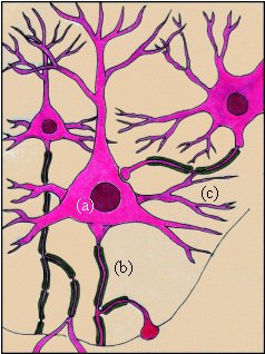
[click to enlarge]
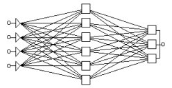
Figure 7. Biological neural tissue. Neural cells (a), axons (b) and dendrites (c) are visible. Where axons touch dendrites or nuclei, synaptic contacts are formed.	Figure 8. Layered artificial neural network. On the left, a pattern is coded. The activation rule propagates the pattern to the right side through the central layer, using the weighted connections. From here, the output can be read. Based on the input-output relation, the learning rule may update the weights

Artificial implementation

Artificial neural networks are simplified models of the biological counterpart. They consist of the following elements:

Processing units (models of neurones)
Weighted interconnections (models of neural connections)
An activation rule, to propagate signals through the network (a model of the signal exchange in biological neurones)
A learning rule (optional), specifying how weights are adjusted on the basis of the established behaviour

The most common ANN are structured in layers (see Figure 8), with an input layer where data is coded as a numeral pattern, one or more hidden layers to store intermediate results, and an output layer that contains the output result of the network.

Neural Network Model Representation

In contrast to symbolic techniques such as decision trees (see link above) the representation of knowledge in a neural network is not easy to comprehend. The set of weights in a network, combined with input and output coding, realises the functional behaviour of the network. As illustrated in Figure 3, such data does not give humans an understanding of the learned model.

Some alternative approaches for representing a neural network are:

Numeric: show the weight matrix; not very informative, but illustrates why a neural network is called sub-symbolic: the knowledge is not represented explicitly, but contained in a distributed representation over many weight factors.
Performance: show that a neural network performs good on the concepts in the data set, even better than other techniques, and do not try to interpret de model
Extract knowledge: techniques exist to extract the model captured in a neural network, e.g. by running a symbolic technique on the same data or by transferring a NN model into an understandable form. Techniques exist to extract statistical models and symbolic models from NN.

more...

Non-parametric Regression (also known as local modelling)

Non-parametric regression¹ belongs to a data analytic methodology usually known as local modelling (Fan, 1995). The basic idea behind local regression consists of obtaining the prediction for a data point x by fitting a parametric function in the neighbourhood of x. This means that these methods are locally parametric as opposed to the methods described in the previous section.

According to Cleveland and Loader (1995) local regression traces back to the 19^th century. These authors provide a historical survey of the work done since then. The modern work on local modelling starts in the 1950s with the kernel methods introduced within the probability density estimation setting (Rosenblatt,1956; Parzen,1962) and within the regression setting (Nadaraya,1964; Watson,1964). Local polynomial regression is a generalisation of this early work on kernel regression. In effect, kernel regression amounts to fitting a polynomial of degree zero (a constant) in a neighbourhood. Summarising, we can state the general goal of local regression as trying to fit a polynomial of degree p around a query point (or test case) x_q using the training data in its neighbourhood. This includes the various available settings like kernel regression (p=0), local linear regression (p=1), etc².

Local regression is strongly related to the work on instance-based learning (e.g. Aha et al.,1991), within the machine learning community. Given a case x for which we want to obtain a prediction, these methods use the training samples that are most similar to x to obtain a local model that is used to obtain the prediction. This type of inductive methodologies do not perform any kind of generalisation of the given data³ and delay learning till prediction time⁴.

Also known as non-parametric smoothing and local regression.
A further generalisation of this set-up consists of using polynomial mixing (Cleveland & Loader,1995), where p can take non-integer values.
This is not completely true for some types of instance-based learners as we will see later. Nevertheless, it is true in the case of local modelling.
That is the reason for also being known as lazy learners (Aha, 1997).

more...

Numerical Values

If a learning algorithm uses numerical values as its example language, it uses a fixed set of attributes with numerical domains to represent the instances of an underlying universe of discourse.

Numerical domains

are not necessarily finite and
have a natural interpretation, that can be used for calculations by a learning algorithm,

which are the two main differences to nominal attribute-value representations, restricting algorithms to distinguish between different values.

more...

On-Line Learning

The learning task here is how to combine advice from several experts.

For instance, several experts predict the weather of the next day by giving a prediction and a probability, e.g. expert₁ says, the probability for rain is 0.8. The prediction of different experts may be conflicting, e.g. expert₂ could say, the probability for rain is 0.2.

The learner then, at the next day, perceives the true outcome, e.g. it actually rains. Hence, the belief in expert₂ decreases, the one in expert₁ increases. The learner again receives predictions of the experts, makes a combination of these advices, in order to decide (e.g. whether or not to take an umbrella), compares its prediction with reality and updates the weights for the experts.

more...

Ontology learning

An ontology is, according to Tom Gruber, "the specification of conceptualizations, used to help programs and humans share knowledge.". In this usage, an ontology is a set of concepts - such as things, events, and relations - that are specified in some way (such as specific natural language) in order to create an agreed-upon vocabulary for exchanging information.

The manual building of ontologies still remains a tedious, cumbersome task which can easily result in a knowledge acquisition bottleneck. The success of the Semantic Web strongly depends on the proliferation of ontologies, which requires that the engineering of ontologies be completed quickly and easily. A method which has proven to be extremely beneficial for the knowledge acquisition task is the integration of knowledge acquisition with machine learning techniques.

more...

Overfitting

Overfitting is the phenomenum that a learning algorithm adapts so well to a training set, that the random disturbances in the training set are included in the model as being meaningful. Consequently (as these disturbances do not reflect the underlying distribution), the performance on the testset (with its own, but definitively other, disturbances) will suffer from techiques that learn to well.

Train and test, cross validation and bootstrap approaches have been developed to cope with this problem.

more...

Prediction of electricity consumption

more...

Prediction of sales

Sales are predicted several weeks ahead in order to minimize stocks.

more...

Prediction of telecommunication services

Prediction of telecommunication services usage at particular day times are helpful in order to minimize the use of external services or optimize network routing.

more...

Preprocessing

Preprocessing cleans, aggregates, discretisizes data, selects and generates features, and handles NULL values in order to pass the data to the data mining tool (modeling step) appropriately.

more...

Principal component analysis

Principal components (or Karhunen-Loeve) directions of the input matrix X are the eigenvectors v_j
The largest principal component of some input data points is the direction that maximizes the variance of the projected data, and the smallest principal component minimizes that variance.

more...

Probabilistic Categorization Tree

The probabilistic categorization tree, used e.g. by COBWEB is a special data structure, a tree where ...

each node defines a cluster, which is a set of (unclassified) examples.
each leaf represents exactly one example, described by an attribute-value tuple.
each inner node represents a cluster, consisting of the union of the clusters of its successors. The other way around: The set of successors partition the set of examples covered by a node.
the root node represents the cluster containing all examples stored in the tree.
for every node n (except for the root node) the following probability is calculated and attached to the node:
Given, that an example from the cluster of n's successor has been drawn under a uniform distribution, how probable is it, that this example is in n's cluster?
for each attribute a, each possible value v of a, and each node n of the tree, the fraction (again interpreted as a probability) of those examples in n's cluster is calculated, where attribute a has value v.

Such a tree is suited for describing a hierarchical clustering probabilistically. This hypothesis language is highly related to the task to achieve

high predictability of variable values, given a cluster, and
high predictiveness of a cluster, given variable values,

by choosing an appropriate tree for a given set of examples.

more...

Probably Approximately Correct (PAC-) Learning

In the PAC-theory the topic is learnability of

concept classes C
over instance spaces LE
by certain hypotheses spaces H,
considering an unknown but fixed probability distribution D over LE, modeling that there is a probability for each instance of LE to occur.

All concepts of the concept classes C and H are subsets of LE.
An example e ∈ LE is classified according to a concept c, if it is given whether e ∈ c or not.

Probably Approximately Correct learnability means, that there is an algorithm A that is able to

select an ε-good hypothesis from H
with a probability of at least 1 - δ
for each δ, ε with 0 < δ < 1/2 , 0 < ε < 1/2.

To find such a hypothesis the algorithm is allowed to read a set X of classified examples, drawn with respect to D.
A hypothesis h is called ε-good, if the probability error_D(h, c) an instance e ∈ LE is drawn and "classified wrong" by h is at most ε:
error_P(h, c) := P(x ∈ (c \ h) ∪ (h \ c))

Two main questions can be distinguished in PAC-theory:

How many examples are needed to learn Probably Approximately Correct?
Is there a polynomal p for a specific concept class C, such that there is an algorithm A, which can find an ε - good hypothesis for each concept c ∈ C with a probability of at least 1 - δ, for each 0 < δ < 1/2 and 0 < ε < 1/2, after having read at most p(1/δ, 1/ε) classified examples from LE, drawn with respect to P ?
How complex is the learning task?
If point 1 is true, is there an algorithm A` and a polynomal p` such that A` can find an ε-good hypothesis in time p`(1 / δ, 1 / ε, |c|), where |c| denotes the representation length of the actual concept c to be learned ?

If question 2 can be answered yes, so can question 1, because in time p`(1/δ, 1/ε, |c|) the cardinality of the set of read examples is bound by a polynomal in 1/δ, 1/ε. more...

PROGOL

The alogorithm PROGOL uses inverted entailment to generalize a set of positive examples with respect to background knowledge B. Examples are definite clauses. Additionally constraints can be given in the form of headless horn clauses.

The outer loop of PROGOL chooses a yet uncovered example, generalizes it to a definite clause and adds that clause to the background knowledge. This is iterated until all examples are covered by the (extended) background knowledge.

The principle of inverting entailment:

For every generalization h of an example e with respect to background knowledge B it is required that B ⋀ h ⊧ e. Applying the deduction theorem leads to B ⋀ ¬ e ⊧ ¬ h. Let ⊥ be the most specific clause, more general (with respect to B) than e. Then B ⋀ ¬ e ⊧ ¬ ⊥ ⊧ ¬ h and h ⊧ ⊥ for all hypotheses h more general than e.

Generalizing one example:

The hypothesis space for the generalization of single examples is a syntactically restricted subset of the set of definite clauses. The restriction is specified by the user via so called "mode declarations", restricting definite clauses in two ways:

The maximal depth i of definite clauses is bound.
The allowed predicate symbols for head and body of the clause are given.

Another indirect restriction of the search space is given by restricting the number of maximal resolution steps when calculating inferences.

There will usually be many possible generalizations of an example. The generalization process can be regarded as a search through a lattice of hypotheses, quasi-ordered by generality.

PROGOL uses θ-subsumption for quasi-ordering the search space.

The most general element of this lattice is the empty clause.
Let ⊥ be the most specific definite clause, such that B ⋀ ⊥ ⋀ ¬ e derives the empty clause in a fixed number of resolution steps.
The most specific element within the user-specified search space is called ⊥_i. It is the the most specific clause of depth at most i, θ-subsuming the clause ⊥.

Within the lattice a top-down search is performed. The description length of clauses serves as a quality measure. The underlying assumption of this approach is, that clauses with shorter representations generalize better than those with longer representations.

For details, please refer to the publication above. more...

Projection Pursuit Regression

Projection pursuit regression (Friedman and Stuetzle, 1981) is a type of additive model (Hastie and Tibshirani, 1990) of the form,

r(x) =

∑

ⁱ⁼¹

f_i (

∑

^j=1

a_jiX_i)

These models can be simply described as additive functions of linear combinations of the attributes. Projection pursuit regression uses the backfitting algorithm (Friedman and Stutzle, 1981) to iteratively obtain the additive terms of the model.

more...

Propositionalisation

The process of of transforming a multi-relational dataset, containing structured examples, into a propositional dataset with derived attribute-value features, describing the structural properties of the examples. The process can thus be thought of as summarising data stored in multiple tables in a single table (the target table) containing one record per example. The aim of this process, of course, is to pre-process multi-relational data for subsequent analysis by attribute-value learners.

more...

Q Learning

Q learning is a method addressing the task of Reinforcement Learning. The main idea is to approximate the function assigning each state-action pair the highest possible payoff.

The setting:

Let

S denote a finite set of states, an agent can be in,
A denote a finite set of actions, an agent may perform,
δ denote a transition function, mapping each state-action pair to a successor state,
r denote a reward function, mapping states-action pairs to payoffs,
and π denote an agent's policy, mapping each state to an action.

Here we use the discounted cumulative reward as a quality measure for fixed policies. For a constant γ ∈ [0, 1] and starting state s₀ this measure is defined as

_∞

V(π) := ∑ γⁱ r_i,

ⁱ⁼⁰

with

s(t) := δ(s(t-1), π(s(t-1))), and
r_i := r(s_i, π(s(t-1))),

∀ t ∈ ℕ^{> 0}.

The method of Q Learning is based on the function Q, defined as followed:

Each state-action pair (s, a) is assgined the highest discounted cumulative reward possible, if state s is the agent's starting state and a is the first action performed. So function Q is based on an optimal policy. If we knew the highest possible discounted cumulative rewards for all possible successor states and actions, then we could calculate the values for the actual state and actions as

Q(s, a) := r(s, a) + γ max Q(δ(s, a), a')

^a'

Of course, an optimal strategy is not known in advance. But it shows that the Q function can be approximated by continously collecting locally observed payoffs and by updating the approximation of Q, using the equation above, although the values for the successor states may have been initialized to arbitrary values.

The Algorithm of Q Learning:

Create a table with an entry for each element in S x A. The entries are referred to by "Q'(s, a)".
Initialize all table entries to 0.
If for a state s and action a a reward r(s, a) and a successor state s' is observed, then update Q'(s, a) as following:

Q'(s, a) := r(s, a) + γ max Q'(s', a')

^a'

It can be shown, that if each state-action transition is passed infinitely often, then the approximation Q' converges to the correct function Q in this finite and deterministic setting. Please refer to the bibliography link above for a proof.

The assumption of passing each state-action transition infinitely often demands, that the agent does not stick to always choosing the action leading to the best payoff, according to the actual approximation of Q, but that it assigns a certain weight to exploring its environment. A possible way of doing so is to define a probability distribution over the set of actions according to the estimation for Q, e.g.

k^{Q'(s, a_i)}

P(a_i | s) =

∑_j k^{Q'(s, a_j)}

for all a_i ∈ A and s ∈ S. This distribution assigns more promising actions a much higher probability of being chosen, but fulfills nonetheless the requirement of passing each possible state-action transition infinitely often.

more...

Quasi-Ordering of Hypothesis Languages

In the concept learning/ILP setting we are looking for a concept, more general than any positive example, and more specific than any concept, covering positive as well as negative examples. So it is a good idea, to structure the hypotheses by their generality, and to generate more general or more specific hypotheses stepwise. The search in a structured search space of all hypotheses can be pruned, which is not possible in an unstructured search space.

In his book "Machine Learning" Tom Mitchell proposed a quasi-ordering for attribute-value hypothesis languages (partial ordering of the set of all hypotheses) based on the more-special-than (or more-general-than) relation:

A concept c₁ is more special than a concept c₂, if and only if every example covered by c₁ is covered by c₂ as well. A concept c₁ is strictly more special than c₂, if it is more special but distinct from c₂, which means that there is at least one instance covered by c₂, that is not covered by c₁ as well.

A concept c₁ is more general than c₂, if c₂ is more special than c₁. Concept c₁ is strictly more general than c₂, if c₂ is strictly more specific than c₁.

If concepts are characterized by attribute values, which can be arranged in a hierarchy according to a more-special-than relation, the search space (which can be seen as a cartesian product of the attribute value sets) can always be (partially) ordered.

more...

RDT

The algorithm RDT basically performs a complete search through a subspace of the hypothesis language of clauses. The subspace results from syntactical restrictions chosen by the user.

The complete search for consistent clauses does not only

guarantee finding a single clause within the search space, if such a clause exists (task of concept learning).
But it also can be used for finding all clauses in the (restricted) hypothesis language, which makes RDT well suited for the characterization task of inductive logic programming.

To perform a complete search, pruning is restricted to cases, where

a general clause does not cover a positive example, so any more specific clause cannot be consistent with the example set, or
a specific clause covers a negative example, so each more general example will do as well.

The search strategy of RDT is top-down induction of horn clauses with rule schemes directing the search. A rule scheme is a clause with at least one predicate variable. Predicate variables are mapped to predicate symbols by substitutions Σ, similar to usual variable substitution, but with the additional restriction that mappings have to be injective, so different predicate variables cannot be replaced by the same predicate symbol.

For rule schemes we can define the "more general than" relation as follows:
Let RS and RS´ be rule schemes. Then RS is more general than RS´ if and only if there are substitutions Σ and σ so that RSΣσ ⊆ RS´.

The search starts with the shortest and therefore most general rule schemes / clauses that only have to be refined by adding literals, if a clause covers positive and negative examples. Redundant literals cannot be added by this strategy.

more...

Regression Functions

A regression function is a function of the form

y = f( x_i, a_I, b) ,

where a prediction of an attribute y depends on the attribute values x_I and a set of parameters a_i.

The most wide spread variant is linear regression, where the function takes the form

y = ∑_i a_i x_i + b

For a specific model the parameters a_i and b are estimated by the learning algorithm, e.g. such, that the empirical error of a test set is minimized.

more...

Regression Rules

Weiss and Indurkhya (1993) have developed a system (SWAP1R) that learns regression rules in a propositional language. The conditional part of the rules consists of a conjunction of tests on the input attributes while the conclusion part contains the associated prediction of the target variable value. Originally these predictions consisted of the average Y value of the cases satisfying the conditional part, but later the possibility of using k-nearest neighbours was added (Weiss & Indurkhya, 1995). This system has the particularity of dealing with regression by transforming it into a classification problem. In effect, the target values of the training cases are pre-processed by grouping them into a set of user-defined bins. These bins act as class labels in the subsequent learning phase. This means that the learning algorithm induces a classification model of the data, where the classes are numbers representing the obtained bins . These numbers can then be used to make numeric predictions for unseen cases. This idea of transforming a regression problem into a classification task was taken further in the work of Torgo and Gama (1996), where a system called RECLA acts as a generic pre-processing tool that allows virtually any classification system to be used in a regression task.

Torgo (1995) has developed a propositional regression rule learner (R2) that also uses an IF-THEN rule format. This algorithm can use several different functional models in the conclusion of the rules . R2 uses a covering algorithm that builds new models while there are uncovered cases to fit. The model is chosen from the model lattice that includes all possible regression models for the conclusion part of the rules. The result of this first step is a rule with empty conditional part and the built model as conclusion. This rule is then specialised by adding conditions to restrict the model domain of applicability with the goal of improving its fit. This restriction is guided by an evaluation function that weighs both the fitting as well as the degree of coverage of the rule. This means that the system is looking for rules with good fit but covering as many cases as possible.

CUBIST is a recent commercial system developed by Ross Quinlan. It learns a set of unordered IF-THEN rules with linear models in the conclusion part. Up to now there is no published work on CUBIST but from our experience with the system it looks like it is a rule-based version of M5 (Quinlan, 1992,1993b). It seems to be a kind of C4.5rules (Quinlan, 1993a) for M5. The system is able to deal with both continuous and nominal variables, and obtains a piecewise linear model of the data. CUBIST can also combine the predictions of this model with k--nearest neighbour predictions (as M5 does).

more...

Regression Trees

Regression trees may be considered as a variant of decision trees, designed to approximate real-valued functions instead of being used for classification tasks.

The inner nodes of regression trees are marked with tests as in decision trees.
The difference is, that the leafs of regression trees may be marked with arbitrary real values, whereas in decision trees the leafs may only be marked with elements of a finite set of nominal values. This makes a real difference only, if you look at sets of trees (e.g. as potential hypotheses languages), instead of comparing single trees.

A further extension is to allow linear functions as labels of leaf nodes. In this case the function at the leaf node reached for a specific example is evaluated for the instance's attribute values, to determine the value of the target attribute. This allows for global approximating by using multiple local approximations.

more...

Reinforcement Learning

In the reinforcement learning scenario the task is to find a policy that maximizes the reward of an agent by experimentation.

more...

Resolution

Resolution provides an important operator for proving clauses.

Let

C₁ := {A₁, A₂, ..., A_m}
C₂ := {¬A₁, B₁, ..., B_n}

be clauses, represented by sets of literals.

Then

D := { A₂, ..., A_m, B₁, ..., B_n }.

can be derived from C₁ and C₂.

Incorporating Substitution

Combining the rule above with substitution leads to an even more powerful resolution rule. This is illustrated by figure 1.

Figure 1: The Resolution-"V".

Let C₁ and C₂ be clauses,

θ₁ and θ₂ be substitutions, and
let L be a literal with
- L ∈ C₁θ₁ and
- ¬L ∈ C₂θ₂.

Then

D := ( C₁θ₁ \ L ) ∪ ( C₂θ₂ \ ¬L )

can be derived from C₁ and C₂.

more...

Restricted First Order Logic

Many machine learning algorithms use a restriction of first order logic as a formalism for representing hypotheses, examples and sometimes background knowledge.

Advantages of choosing logical representations are:

Representations are readable by humans.
Logic is a well-understood mathematical discipline, so a plenty of mathematical results can be used, searching for learning methods and proving their correctness.
Examples, hypotheses and background knowledge can be expressed within the same formalism.

A problem of full first order logic is that it is algorithmically hard to check whether a formula implies another, which is necessary for finding hypotheses that are consistent with the set of examples. To receive a more tractable formalism, restrictions of first order logic are chosen. Depending on how expressive the restriction has to be, one can choose between

propositional logic
horn clauses
function-free clauses
non-recursive clauses

and many more specific restrictions.

If e.g.

background knowledge is given in the form of function-free ground facts (relational database),
function-free horn clauses are sufficient as the hypothesis language for a specific learning task,
then a possible candidate for an inference operator is the (in the general case incomplete) θ-subsumption.

This restriction of first order logic is much more tractable and therefore to be preferred (if it is expressive enough).

Typical restrictions of the hypothesis language are variously restricted clauses, e.g. function-free horn clauses. more...

Revision

The learning task is to revise a given theory, in order to no longer imply a given set of unwanted facts. In other words, a theory has become inconsistent and shall be adjusted to some new insights.

An obvious demand is, that adjustment should not change more of the theory than necessary. In particular, parts that are not concerned in the derivation of the incorrect logical facts should not be changed at all.

more...

Sampling

Sampling is the process of selecting a proper subset of elements from the full population so that the subset can be used to make inference to the population as a whole. A probability sample is one in which each element has a known and positive chance (probability) of selection. A simple random sample is one in which each member has the same chance of selection.

more...

Searching Version Spaces

If we can manage to find an appropriate ordering of our hypothesis language, then learning can be regarded as navigating through version spaces, with each new example read limiting the number of hypotheses, that are still consistent.

The search will either lead from specific to general, driven by positive examples (bottom-up), or from general to specific, driven by negative examples (top-down).

The CANDIDATE-ELIMINATION Algorithm combines a bottom-up and a top-down search.

more...

Sequence Prediction

The scenario for the task of Sequence Prediction is the following.

Given: Sequences of events, e.g. in the form (E₁, t₁), (E₂, t₂), ..., (E_n, t_n), where the E_i denote events, and the t_i denote points in time.

The target is to find rules, accurately predicting the occurence of future events, given the event sequence up to the actual point in time.

more...

Sequences and episodes

more...

Spatial relationships

A relationship in spatial data is a relationship between features in a Euclidean space, defined in terms of the co-locational trends of two or more features over that space. An example is determining the confidence of the ‘where there’s smoke there’s fire’ with respect to a set of coordinates, each representing the feature smoke or fire. The task here would be to determine whether fire occurs in the neighborhood of smoke more than is randomly likely.

The treatment of relationships among spatial objects is an essential task in geographic data processing and CAD/CAM. more...

Star

The Star method is suitable for the task of concept learning as well as for conceptual clustering. It can deal with different kinds of attribute-value representations of examples. The idea is to find all most general descriptions, that separate an example set from other example sets. Then, according to a certain preference criterion, the best of all descriptions is chosen. The concepts or clusters generated that way may be specialized afterwards, to make them disjoint.

Let P denote a set of instances to be covered and N a set of instances that should not be covered.
A partial star is a conjunction of conditions testing attribute-values.
Such a partial star is called consistent with P and N, if it covers every p ∈ P, but no n ∈ N.

STAR(P|N), the star of P against N, is defined as the disjunction of all maximally general partial stars, consistent with P and N.

As a quality measure for stars and partial stars, a so called "Lexical Evaluation Function" (LEF) is used.

For algorithms based on the star-method, it is often sufficient to build stars of single instances of the example language against a set of examples.

Let

p be an instance to be covered,
N be a set of instances that should not be covered,
s be a parameter for bounding complexity.

How to generate STAR({p}|N,s):

Generate a list of partial stars with exactly one condition, taken from p. These partial stars may still cover an n ∈ N, and therefore be inconsistent.
If there are more than s partial stars in the list, remove all, except from the best s ones, according to the LEF.
As long as there are inconsistent partial stars, that can be extended by adding a conjunction, such that the result has not been generated before, do:
- Extend all inconsistent partial stars by one condition and add them to the list.
- If the list contains more than s elements, just keep the best s ones.
Remove all inconsistent partial stars from the list.
Output the list, ordered by the LEF.

more...

Statistical Learning

The statistical learning theory focusses on two major questions:

Asymptotic Analysis: Can it be proven, that with an increasing number of examples the empirical error converges to the real error?
Learning Rate: If point 1 has been proved, then how fast does the empirical error converge to the real error?

more...

Support Vector Machine (SVM)

Support vector machines were developed by Vapnik et al. based on the Structural Risk Minimization principle from statistical learning theory. They can be applied to regression, classification, and density estimation problems.

Vapnik's book "Statistical Learning Theory" is listed under "Publications", above.
Focussing on classification, SVMs take as input an i.i.d. training sample S_n

(x₁,y₁), (x₂,y₂), ..., (x_n,y_n)

of size n from a fixed but unknown distribution Pr(x,y) describing the learning task. x_i represents the document content and y_i ∈ {-1,+1} indicates the class.

In their basic form, SVM classifiers learn binary, linear decision rules

h(x) = sign(w *x + b) =

+1, if w * x + b > 0, and
-1, else

described by a weight vector w and a threshold b. According to which side of the hyperplane the attribute vector x lies on, it is classified into class +1 or -1. The idea of structural risk minimization is to find a hypothesis h for which one can guarantee the lowest probability of error. For SVMs, Vapnik shows that this goal can be translated into finding the hyperplane with maximum margin for separable data, this is depicted in the following figure.

For separable training sets SVMs find the hyperplane h, which separates the positive and negative training examples with maximum margin. The examples closest to the hyperplane are called Support Vectors (marked with circles).

Computing this hyperplane is equivalent to solving the following quadratic optimization problem (see also algorithms).

minimize: W(α) =

n n n

- ∑ α_i + 1/2 * ∑ ∑ y_iy_jα_iα _j(x_i * x_j)

i=1 i=1 j=1

subject to:

n n

∑ y_iα_i = 0, ∀ : 0 < α_i < C

i=1 i=1

Support vectors are those training examples x_i with α_i > 0 at the solution. From the solution of this optimization problem the decision rule can be computed as

n

w * x = ∑ α_iy_i (x_i * x) and b = y_usv - w * x_usv

i=1

The training example (x_usv,y_usv) for calculating b must be a support vector with α_usv < C.

For both solving the quadratic optimization problem as well as applying the learned decision rule, it is sufficient to be able to calculate inner products between document vectors. Exploiting this property, Boser et al. introduced the use of kernels K(x₁,x₂) for learning non-linear decision rules.

Popular kernel functions are:

K_poly (d₁,d₂) = (d₁ * d₂ + 1)^d

K_rbf (d₁,d₂) = exp(γ (d₁ - d₂)² )

K_sigmoid (d₁,d₂) = tanh( s(d₁ * d₂) + c )

Depending on the type of kernel function, SVMs learn polynomial classifiers, radial basis function (RBF) classifiers, or two layer sigmoid neural nets. Such kernels calculate an inner-product in some feature space and replace the inner-product in the formulas above.

A good tutorial on SVMs for classification is "A Tutorial on Support Vector Machines for Pattern Recognition", for details, please follow the corresponding link above. more...

SVM for regression

SVMs can be adapted for regression with a quantitative response, in ways that inherit some of the properties of the SVM classifier.

more...

SVM light

SVM^light is an implementation of Support Vector Machines (SVMs) in C.

The main features of the program are the following:

fast optimization algorithm

working set selection based on steepest feasible descent
"shrinking" heuristic
caching of kernel evaluations
use of folding in the linear case

includes algorithm for approximately training large transductive SVMs (TSVMs)
can train SVMs with cost models
handles many thousands of support vectors
handles several ten-thousands of training examples
supports standard kernel functions and lets you define your own
uses sparse vector representation

The source code is free for scientific use. Please follow the link "SVM^light - Details and Download". There is also a regression support vector machine based on SVM^light available: Please follow the link labeled "mySVM".

Description

SVM^light is an implementation of Vapnik's Support Vector Machine (see "The Nature of Statistical Learning Theory") for the problem of pattern recognition. The optimization algorithm used in SVM^light is described in "Making large-Scale SVM Learning Practical.". The algorithm has scalable memory requirements and can handle problems with many thousands of support vectors efficiently. This new version also includes a new algorithm for training large-scale transductive SVMs. The algorithm proceeds by solving a sequence of optimization problems lower-bounding the solution using a form of local search.

The code has been used on a large range of problems, including text classification (see publications above), several image recognition tasks, and medical applications. Many tasks have the property of sparse instance vectors. This implementation makes use of this property which leads to a very compact and efficient representation.

more...

Syntax/Grammar/Automata - Learning

Given:

an infinite stream of examples, where examples are either
- well-formed sentences of a language, or
- sentences classified as well-formed or not well-formed,
and
- a class of languages ₤, where for each language there exists a procedure to decide whether a sentence is member of this language,
- or a class of automata Å, where each automata can decide whether a given sentence is accepted.

Find the language L ∈ ₤ / the automaton A ∈ Å, that generates / accepts all well-formed sentences.

The most interesting language, of course, is natural language. However, most methods learn much more restricted classes of languages, e.g. pattern languages (i.e. sets of strings).

more...

Telecommunications

Call Center Application more...

Text categorisation

more...

Theta-Subsumption

The θ-subsumtion is a correct, but incomplete inference operator for clauses with the advantage of being feasible, while correct and complete inference operators in full first order logic are known to be algorithmically intractable.

A clause C₁ θ-subsumes another clause C₂, if and only if a substitution θ exists, such that C₁θ ⊆ C₂.
If C₁ θ-subsumes C₂ then C₁ implies C₂.

Θ-subsumption may also be used for quasi-ordering the hypothesis language of clauses. more...

Theta-Subsumption Ordering

When searching the hypothesis space of clauses, one possible feasible way to quasi-order the hypothesis space is to use θ-subsumption. The general idea is to structure the search space with respect to generality of instances. Intuitively the following definition of "more general than" is reasonable: If c and c' are clauses and c ⊨ c' then c is more general than c'.

However, it is more feasible to define the "more general than"-relation by restricting inference to θ-subsumption. Let C₁ and C₂ be clauses. Then C₁ is more general than C₂, if and only if:
There is a substitution θ, such that C₁θ ⊆ C₂ .

more...

Time Series Analysis

The general task

Given are time series, which are ordered sets of observations { x₁, .., x_n }, where x_i denotes the observation at point i in time, e.g. a real-valued vector.

The goal is to predict the behaviour at point n+1 in time, which possibly may be determined by a function.

More special tasks

Given: time series

Trend:	Find a characterization of the direction of change over time.
Level Change:	Find points in time, from where on the overall level of observeable values will change.
Cycles:	Find cycles in the sequence of changes over time.

more...

Time series clustering and indexing

more...

Top-Down Induction of Decision Trees (TDIDT)

Top-down induction of decision trees is a method for the task of concept learning (supervised learning).

Given:
A set of classified examples in attribute-value representation, where the set of classes is finite.

The Method:
A decision tree is constructed top-down. In each step a test for the actual node is chosen (starting with the root node), which best seperates the given examples by classes. The quality of a test is measured by the impurity / variance of example sets. The most common measure is the information gain.

A test is a mapping from the set of all instances of the underlying example language to a finite set of possible results. In the decision tree there is a successor of the actual node for each possible result of the test. The given set of examples is split with respect to the chosen test. For each successor that does not meet a given acceptance criterion, e.g. that all examples are of the same class, the procedure is started recursively.

Often the set of possible tests is limited to splitting the examples according to the value of a certain attribute, so the method is restricted to choosing a good attribute for each inner node. If numerical attribute values are incorporated, tests may compare the value of certain attributes to appropriate constants.

The aim of top-down induction of decision trees is to find a decision tree that is as small as possible and fits the data, because it is assumed that it is likely to find a good generalization of the training data that way. more...

Top-Down Induction of Horn Clauses

In Inductive Logic Programming a common method for

finding a horn clause that covers as much instances of a set of positive examples as possible,
but does not cover any instance of a set of negative examples

is to use a general-to-specific search through a given hypothesis language.

General-to-specific search for horn clauses:

Given a set of examples, a specific target predicate P and its arity, e.g. 2.
Start with a most general horn clause with predicate P in the head. These are the horn clauses with empty bodies and different variables at each component of P, e.g. " P(x, y) ← ".
These clauses are most general, because they derive P(x, y) for every possible substitution of x and y.
In general there will be negative examples in the example set, which then will be covered by all most general clauses. In this case, the actual horn clause is refined step by step, until no negative example is covered any more. This is done by adding further conditions to the clause's body. Doing so decreases the set of substitutions fulfilling all conditions of the horn clause, so the clause becomes more specific.

Depending on the refinement procedure two approaches can be distinguished:

The refinement procedure can be guided heuristically, as done by FOIL (not restricted to horn clauses) to construct a clause that covers as many of the yet uncovered positive, but none of the negative examples.
Another way is to perform a complete search through a syntactically restricted hypothesis space, which will generally require higher computational efforts. On the other hand, it enables to give guarantees, e.g. that a most general solution in the hypothesis space is found. An algorithm following this approach is RDT.

more...

Top-Down Induction of Regression Trees

The Top-Down Induction of Regression Trees addresses the task of function approximation. Nevertheless the method is quite similar to top-down induction of decision trees.

Given:

a set E of instances of the examples language in attribute-value representation
for each instance x ∈ E its function value f(x)

The method:

A regression tree is constructed top-down.

In each step a test for the actual node is chosen (starting with the root node). The search for good tests is guided by variably defined quality measures, which reward tests that induce partitions which subsume instances with similar function values.
As in decision trees in regression trees a test is a mapping from the set of all instances of the underlying example language to a finite set of possible results. There is a successor of the actual node for each possible result of the test.
The given set of examples is split with respect to the chosen test.
For each successor that does not meet a given acceptance criterion, the procedure is called recursively.
Each leaf of a regression tree is marked by a real value. The value is, of course, chosen such, that the actual quality measure for the leaf is maximized. Alternatively a linear function may be attached to leaf nodes, if the attributes describing examples are numerical as well.

When the method of regression trees is invoked, there are often numerical attribute values, and tests may compare the value of certain attributes to appropriate constants.

The aim of regression trees usually is to find a good generalization of the training data, which means good predictions of yet unseen values of the actual function. Another possible aim is to analyze which variables are well suited to predict a target value. more...

Train and Test

Keeping a test set additionally to the train set is a general method to estimate the accuracy of a concept learning algorithm (classifier). Given a sample of classified instances and a concept learning algorithm, this is how this method works:

Split the data in two parts, a training set and a test set.
Run the learner on the training set, but do not show the test set. Let h denote the hypothesis output by the learner.
Use h to classify all instances of the test set. The fraction of correct classified instances is the estimated accuracy.

Usually a fraction of 20-30% of the available data is chosen as the test set. This is a good option, if the size of the test set is larger than 1000.

more...

VC dimension

The VC dimension (for Vapnik Chervonenkis dimension) is a measure of the capacity of a classification algorithm. It is one of the core concepts in statistical learning theory. It was originally defined by Vladimir Vapnik and Alexey Chervonenkis.

Intuitively, the capacity of a classification model is related to how complicated it can be. Think of thresholding a high-degree polynomial, where if the polynomial evaluates above zero, we classify that point into a positive class, negative otherwise.

If we use a very high-degree polynomial, it can be very wiggly, and can fit a training set exactly. But, we should expect that outside of the training points, the classifier would not generalize well, because it is too wiggly. Such a polynomial has a high capacity. Alternatively, we can think about thresholding a linear polynomial. This polynomial may not fit the entire training set, because it has a low capacity. This notion of capacity can be made more rigorous.

First, we need the concept of shattering. Consider a classification model f with some parameter vector θ. The model f can shatter a set of data points if, for all assignments of labels to those data points, there exists a θ such that the model f makes no errors when evaluating that set of data points. more...

Version Space

Version Spaces may be regarded as a method or as a hypothesis language itself.

In concept learning one has

a set of classified examples and
a set of hypotheses, which define the possible results of the algorithm.

The task of incremental concept learning demands, that the learning algorithm reads one example per iteration and outputs a hypothesis each time. It can be assumed that the algorithm may not store many of the seen examples, but basically just revises the actual hypothesis according to the actual example.

One often has several different hypotheses fitting the data, and it can be an advantage, for reasons of efficiency, to define a preference criterion, to have a unique hypothesis at each point in time.

But in fact there often is a set of possible results, fitting the data, which we expect to become smaller, the more examples the algorithm has read. By using Version Spaces, one can avoid to choose a preference criterion, which may not be justified in some situations, and instead represent the set of all hypotheses of an underlying hypotheses language that (still) fit the data. After each iteration step an arbitrary element of the represented set of hypotheses can be chosen as an output of the learning algorithm.

The representation of the set can be achieved by half-ordering the hypotheses language and by storing just the most general and the most specific hypotheses.

more...

Web usage mining

Web mining is the integration of information gathered by traditional data mining methodologies and techniques with information gathered over the World Wide Web. Web mining is used to understand customer behavior, evaluate the effectiveness of a particular Web site, and help quantify the success of a marketing campaign.

Web mining allows you to look for patterns in data through content mining, structure mining, and usage mining. Content mining is used to examine data collected by search engines and Web spiders. Structure mining is used to examine data related to the structure of a particular Web site and usage mining is used to examine data related to a particular user's browser as well as data gathered by forms the user may have submitted during Web transactions.

The information gathered through Web mining is evaluated (sometimes with the aid of software graphing applications) by using traditional data mining parameters such as clustering and classification, association, and examination of sequential patterns. more...

WEIGHTED-MAJORITY

The WEIGHTED-MAJORITY algorithm addresses the task of on-line learning. Given a set of prediction rules (or advice from several experts), the algorithm maintains a weight for each rule (or expert), specifying how to form the algorithm's prediction from the set of predictions.

The algorithm runs in rounds. Every round

the predictions of all rules are calculated first, and
compared to the real outcome in step 2.
Step 3 is to update the weights. This is done by decreasing the weights of rules that predicted wrong.

So the algorithm favours rules with high accuracy.
Every round a prediction is made, before the real outcome can be observed. The aim is to make as few mistakes as possible.

Let

w_i denote the weight of rule i,
n denote the number of rules, and
H_i(e) denote the prediction of rule number i for example e.

The algorithm for a binary prediction task, where the task is to predict if 0 or 1, e.g. if an instance belongs to a concept or not, or if it will rain tomorrow:

For i = 1 to n do: w_i = 1
Repeat
- Read an unclassified example e.
- W₀ = Σ_{i:Hi(x)=0}w_i
- W₁ = Σ_{i:Hi(x)=1}w_i
- If (W₀ > W₁) output prediction 0.
- If (W₀ < W₁) output prediction 1.
- If (W₀ = W₁) output a random prediction.
- Compare the prediction of every single rule with the true outcome, and for each rule i that predicted wrong:
  w_i = β * w_i, with β ∈ [0, 1[.

β is a fixed parameter, specifying how drastically to punish wrong predictions. By choosing β = 0 we receive the CANDIDATE-ELIMINATION algorithm, where each hypothesis inconsistent with an example is permanently deleted.

more...

WEKA

Weka is a collection of machine learning algorithms for solving real-world data mining problems. It is written in Java and runs on almost any platform. The algorithms can either be applied directly to a dataset or called from your own Java code. Weka is also well-suited for developing new machine learning schemes. Weka is open source software issued under the GNU public license.

more...